- Workshop 2024 Running the first experiment on TeraStat 2 (Antonio Mastrandrea, Emanuele Corti)
-
Running the first experiment on TeraStat 2
Author
Dott. Antonio Mastrandrea, Dott. Emanuele Corti (supercalcolo.dss@uniroma1.it)
In this activity, are introduced the steps required to perform a simple experiment on TeraStat2.
A copy of the materials used for this case study is available for download here
- Workshop 2024 Case 1: Leveraging the multi-core capabilities of a super-computing cluster to train Machine Learning models in R (Pierfrancesco Alaimo Di Loro)
-
Leveraging the multi-core capabilities of a super-computing cluster to train Machine Learning models in R
Author
Prof. Pierfrancesco Alaimo Di Loro (p.alaimodiloro@lumsa.it)
Problem Statement
The recent strides in super-computing technology have shifted the focus from “slim” statical models to “brute-force” algorithmic routines that leverage the new computational capabilities to learn unstructured patterns from huge amounts of data. Versatile Machine Learning methods now have the upper hand in solving many real-world challenges but their practical application within reasonable time frames demands exploitation of all the available computational resources. This necessity becomes particularly pronounced when ensuring robust validation and uncertainty quantification through resampling techniques like cross-validation and bootstrap, which require training the same model a (sometimes large) number of times. The naive sequential implementation of these techniques grows linearly with the number of resamples - a highly inefficient approach. Considering that such operations can be executed independently, we propose harnessing the distributed architecture of TeraStat2 via R to perform them in parallel on multiple cores. This can significantly reduce the overall execution time whenever the cost of each single operation is sufficiently large.
K-fold Cross-Validation
K-fold cross-validation requires splitting the training data into K non-overlapping subsets of data. The model is to be trained K times. Every time, one of the subset is held-out from the training process and used to test the predictive performance of the model trained on the remaining K−1 subsets. When the training of the model is computationally expensive and K grows large, performing such operation sequentially might become unfeasible. Leveraging multi-trheading using all the available cores to perform the multiple trainings in parallel can be extremely profitable. More details are provided in the slides.
Bootstrapping for uncertainty quantification
The problem of quantifying prediction uncertainty in non-parametric models is usually addressed using the non-parametric bootstrap approach, which can be quite accurate in data-rich settings. This approach consists in resampling the data an arbitrary number of times B (generally >100 ) and training the model on each of the resampled datasets. The B models’ fits are an approximation of the model distribution when the training set is sampled from the data empirical distribution. They can be used to quantify the model variance and the sum of model bias and sampling noise. This procedure requires fitting the same model a quite large number of times (B ) and, when each single fit is computationall expensive, it can become unfeasible to be performed sequentially. More details are provided in the slides.
Proposed solution
A copy of the code used in the following solutions can be downloaded from here
K-fold Cross-Validation
The Rcode XGBoost_ErrorValidation_Locale.R (that can be ran in locale) provides examples of when multi-threading is not profitable and when it is profitable, given that enough computational power is available. We consider the Extreme Gradient Boosting machine learning model and the agaricus data from the package.
# Packages ----------------------------------------------------------------

require(tidyverse)
require(xgboost)
require(pROC)
require(microbenchmark)
require(doParallel)
require(parallel)
require(foreach)

# Loading data ------------------------------------------------------------

# We consider the agaricus.train and agaricus.test data from the xgboost package
data("agaricus.train")
data("agaricus.test")

# Each object is a list of: data (covariates), labels (outcome)
# Covariates
Xtr <- agaricus.train$data %>% as.matrix()
head(Xtr)
Xte <- agaricus.test$data %>% as.matrix()
head(Xte)
# Outcome
Ytr <- agaricus.train$label
Yte <- agaricus.test$label
table(Ytr)
table(Yte)
# Classification task


# Single XGboost fit ------------------------------------------------------

# We focus only on the training data
# We keep al parameters to default, but specify eta=0.01, nrounds=10
eta.our <- 0.01
nround.our <- 10

# TRAINING
oo <- xgboost(data = Xtr, label = Ytr,
              eta=eta.our, nrounds = nround.our,
              eval_metric = "auc", nthread=1)

# PREDICTING
ooPreds.tr <- predict(oo, Xtr)
pROC::auc(Ytr, ooPreds.tr, direction="<")

ooPreds.te <- predict(oo, Xte)
pROC::auc(Yte, ooPreds.te, direction="<")

# Time required on 1 thread
microbenchmark(xgboost(data = Xtr, label = Ytr,
                       eta=eta.our, nrounds = nround.our,
                       eval_metric = "auc",
                       verbose = F, nthread=1))
# Each training costs approximately 210 milliseconds


# K-fold cross-validation for error evaluation  --------------------------------------

# If we perform K-fold cross-validation, we must fit the model K times
# We can do it sequentially, or in parallel
# Sequentially, the fitting time is (approximately) multiplied by K

# Let's try with K=10
K <- 10
# Assign each unit to a different fold, at random
set.seed(130494)
foldsids <- sample(1:K, size=nrow(Xtr), replace = T)


# SEQUENTIAL
# We use the "foreach" command to loop across folds
foreach(k=1:K, .combine = c) %do% {

  # Fit on all train but k-th fold
  oonow <- xgboost(data = Xtr[foldsids!=k,], label = Ytr[foldsids!=k],
                   eta=eta.our, nrounds = nround.our,
                   eval_metric = "auc",
                   verbose = F, nthread=1)

  # Predict on the k-th fold
  preds.now <- predict(oonow, Xtr[foldsids==k,])

  # Evaluate AUC
  auc(Ytr[foldsids==k], preds.now, direction="<", quiet = T)
}

# PARALLEL
# We set up parallel computation use the "foreach" command with %dopar%

# Available cores
avcores <- parallel::detectCores()-1  # We always keep 1 spare core
ncores <- min(K, avcores)             # We do not parallelize more than we need

#########################
##### WINDOWS ONLY  #####
#########################
cl <- parallel::makeCluster(ncores)   # On Windows we set-up the cluster
doParallel::registerDoParallel(cl)    # Registers parallel cluster
clusterExport(cl = cl, c("Xtr", "Ytr", "K", "eta.our", "nround.our"),
              envir = .GlobalEnv)
clusterEvalQ(cl, library("xgboost"))
clusterEvalQ(cl, library("pROC"))

# We use the "foreach" command to loop across folds
foreach(k=1:K, .combine = c) %dopar% {

  # Fit on all train but k-th fold
  oonow <- xgboost(data = Xtr[foldsids!=k,], label = Ytr[foldsids!=k],
                   eta=eta.our, nrounds = nround.our,
                   eval_metric = "auc", verbose = F)

  # Predict on the k-th fold
  preds.now <- predict(oonow, Xtr[foldsids==k,])

  # Evaluate AUC
  auc(Ytr[foldsids==k], preds.now, direction="<", quiet = T)
}

stopCluster(cl)
#########################
#########################
#########################

# #################
# ##### UNIX  #####
# #################
# # We use the "mclapply" command to loop across folds
# mclapply(1:K,
#          function(k){
#
#            # Fit on all train but k-th fold
#            oonow <- xgboost(data = Xtr[foldsids!=k,], label = Ytr[foldsids!=k],
#                             eta=eta.our, nrounds = nround.our,
#                             eval_metric = "auc", verbose = F)
#
#            # Predict on the k-th fold
#            preds.now <- predict(oonow, Xtr[foldsids==k,])
#
#            # Evaluate AUC
#            auc(Ytr[foldsids==k], preds.now, direction="<", quiet = T)
#          },
#          mc.cores = ncores) %>% unlist()
#
# #########################
# #########################
# #########################


# LET'S COMPARE THE EXECUTION TIMES: 10 tries to keep it short

# SEQUENTIAL
microbenchmark({
  foreach(k=1:K, .combine = c) %do% {

    # Fit on all train but k-th fold
    oonow <- xgboost(data = Xtr[foldsids!=k,], label = Ytr[foldsids!=k],
                     eta=eta.our, nrounds = nround.our,
                     eval_metric = "auc",
                     verbose = F, nthread=1)

    # Predict on the k-th fold
    preds.now <- predict(oonow, Xtr[foldsids==k,])

    # Evaluate AUC
    auc(Ytr[foldsids==k], preds.now, direction="<", quiet = T)
  }
}, times=10)
# It is (210*(9/10))*10ms = 1.89secs: 10 times the fit on 9/10 of the data (approx)

# PARALLEL
microbenchmark({
  #########################
  ##### WINDOWS ONLY  #####
  #########################
  cl <- parallel::makeCluster(ncores)   # On Windows we set-up the cluster
  doParallel::registerDoParallel(cl)    # Registers parallel cluster
  clusterExport(cl = cl, c("Xtr", "Ytr", "K", "eta.our", "nround.our"),
                envir = .GlobalEnv)
  clusterEvalQ(cl, library("xgboost"))
  clusterEvalQ(cl, library("pROC"))

  # We use the "foreach" command to loop across folds
  foreach(k=1:K, .combine = c) %dopar% {

    # Fit on all train but k-th fold
    oonow <- xgboost(data = Xtr[foldsids!=k,], label = Ytr[foldsids!=k],
                     eta=eta.our, nrounds = nround.our,
                     eval_metric = "auc",
                     verbose = F, nthread=1)

    # Predict on the k-th fold
    preds.now <- predict(oonow, Xtr[foldsids==k,])

    # Evaluate AUC
    auc(Ytr[foldsids==k], preds.now, direction="<", quiet = T)
  }

  stopCluster(cl)
  #########################
  #########################
  #########################

  # #################
  # ##### UNIX  #####
  # #################
  # mclapply(1:K,
  #          function(k){
  #
  #            # Fit on all train but k-th fold
  #            oonow <- xgboost(data = Xtr[foldsids!=k,], label = Ytr[foldsids!=k],
  #                             eta=eta.our, nrounds = nround.our,
  #                             eval_metric = "auc", verbose = F)
  #
  #            # Predict on the k-th fold
  #            preds.now <- predict(oonow, Xtr[foldsids==k,])
  #
  #            # Evaluate AUC
  #            auc(Ytr[foldsids==k], preds.now, direction="<", quiet = T)
  #          },
  #          mc.cores = ncores) %>% unlist()
  #
  # #########################
  # #########################
  # #########################
}, times=10)

# Approximately 2.84 seconds
# Not really convenient... It took longer than sequentially!
# This is because the overhead of multithreading is more than the gain from parallel execution

# The overhead sensibly impact the performances when:
# 1. Each single operation is not really expensive
# 2. We are not executing many operations in parallel
# 3. Proportion of serial and parallelized code

# In practice: n_k*K < n_k+c_p, where c_p is the cost of parallelization


# Longer fit and more loops -----------------------------------------

# New parameters
eta.our2 <- 0.001   # Less learning
nround.our2 <- 100  # More iterations
max.depth2 <- 10    # Longer trees
subsample2 <- 0.7   # Use more data

# Time required
microbenchmark(xgboost(data = Xtr, label = Ytr,
                       eta=eta.our2, nrounds = nround.our2,
                       max.depth=max.depth2, subsample=subsample2,
                       eval_metric = "auc",
                       verbose = F, nthread=1), times=10)
# Approximately 2.5 seconds

# If K-fold cross validation with K=15
K <- 15
set.seed(130494)
foldsids <- sample(1:K, size=nrow(Xtr), replace = T)

# If we perform K-fold cross-validation sequentially, the time would be approximately
# 2.5*15*14/15 seconds = 35 secs (approx)

# SEQUENTIAL
t0 <- proc.time()
foreach(k=1:K, .combine = c) %do% {

  # Fit on all train but k-th fold
  oonow <- xgboost(data = Xtr[foldsids!=k,], label = Ytr[foldsids!=k],
                   eta=eta.our2, nrounds = nround.our2,
                   max.depth=max.depth2, subsample=subsample2,
                   eval_metric = "auc",
                   verbose = F, nthread=1)

  # Predict on the k-th fold
  preds.now <- predict(oonow, Xtr[foldsids==k,])

  # Evaluate AUC
  auc(Ytr[foldsids==k], preds.now, direction="<", quiet = T)
}
(tlag <- proc.time()-t0)
# Approximately 35 seconds indeed

# PARALLEL
# Using K cores on my machine it should take
# (2.5*15*14/15)/15 + c_p = 2.3 secs + c_p

# Set number of cores
ncores <- min(K, avcores)             # We do not parallelize more than we need

t0 <- proc.time()

#########################
##### WINDOWS ONLY  #####
#########################
avcores <- parallel::detectCores()-1  # We always keep 1 spare core
ncores <- min(K, avcores)             # We do not parallelize more than we need
cl <- parallel::makeCluster(ncores)   # On Windows we set-up the cluster
doParallel::registerDoParallel(cl)    # Registers parallel cluster

n <- nrow(Xtr)
clusterExport(cl = cl,
              c("Xtr", "Ytr", "eta.our2", "nround.our2", "max.depth2", "subsample2"),
              envir = .GlobalEnv)
clusterEvalQ(cl, library("xgboost"))
clusterEvalQ(cl, library("pROC"))

# We use the "foreach" command to loop across folds
foreach(k=1:K, .combine = c) %dopar% {
    # Fit on all train but k-th fold
  oonow <- xgboost(data = Xtr[foldsids!=k,], label = Ytr[foldsids!=k],
                   eta=eta.our2, nrounds = nround.our2,
                   max.depth=max.depth2, subsample=subsample2,
                   eval_metric = "auc",
                   verbose = F, nthread=1)

  # Predict on the k-th fold
  preds.now <- predict(oonow, Xtr[foldsids==k,])

  # Evaluate AUC
  auc(Ytr[foldsids==k], preds.now, direction="<", quiet = T)
}

stopCluster(cl)
#########################
#########################
#########################

# #################
# ##### UNIX  #####
# #################
# mclapply(k=1:K,
#          function(k){
#            # Fit on all train but k-th fold
#            oonow <- xgboost(data = Xtr[foldsids!=k,], label = Ytr[foldsids!=k],
#                             eta=eta.our2, nrounds = nround.our2,
#                             max.depth=max.depth2, subsample=subsample2,
#                             eval_metric = "auc",
#                             verbose = F, nthread=1)
#
#            # Predict on the k-th fold
#            preds.now <- predict(oonow, Xtr[foldsids==k,])
#
#            # Evaluate AUC
#            auc(Ytr[foldsids==k], preds.now, direction="<", quiet = T)
#          },
#          mc.cores = ncores)
# #########################
# #########################
# #########################

(tlag <- proc.time()-t0)

# 7-8 seconds!


# LOO cross-validation for error evaluation  --------------------------------------

# If we perform LOO cross-validation, we must fit the model n times
# No way we are doing this sequentially, indeed the time would be approximately
# 2.5*6500 seconds = 4hours 30 mins

# We can try this in parallel
# On the 19 cores of my machine it should take
# 2.5*6500/19 + c_p = 14 mins + c_p

# Still too long to do here...
# What if we do it on Terastat?
The Rcode XGBoost_ErrorValidation_Terastat.R shows an example of when leveraging the multi-core capabilities of a super-computing cluster becomes necessary to improve on the advantages guaranteed by multi-threading. We consider the Extreme Gradient Boosting machine learning model and the agaricus data from the package. Make sure all the required packages are installed before running.
# Packages ----------------------------------------------------------------

require(tidyverse)
require(xgboost)
require(pROC)
require(doParallel)
require(parallel)
require(foreach)
require(microbenchmark)

# Loading data ------------------------------------------------------------

# We consider the agaricus.train data from the xgboost package
data("agaricus.train")

# Each object is a list of: data (covariates), labels (outcome)
# Covariates
Xtr <- agaricus.train$data %>% as.matrix()
# Outcome
Ytr <- agaricus.train$label


# Setting-up single run -----------------------------------------

# XGBoost parameters
eta.our <- 0.001   # Less learning
nround.our <- 100  # More iterations
max.depth.our <- 10    # Longer trees
subsample.our <- 0.7   # Use more data

# Time required
print("Time required by one single run")
microbenchmark(xgboost(data = Xtr, label = Ytr,
                       eta=eta.our, nrounds = nround.our,
                       max.depth=max.depth.our, subsample=subsample.our,
                       eval_metric = "auc",
                       verbose = F, nthread=1), times=10)


# LOO parallelcross-validation for error evaluation  --------------------------------------

# We are looping over all n rows of the data
n <- nrow(Xtr)

# Number of cores
avcores <- parallel::detectCores()-1    # We always keep 1 spare core
ncores <- min(n, avcores)               # We do not parallelize more than we need

t0 <- proc.time()
preds.loo <- mclapply(1:n,
                      function(i){
                        # Fit on all train but i-th obs
                        oonow <- xgboost(data = Xtr[-i,], label = Ytr[-i],
                                         eta=eta.our, nrounds = nround.our,
                                         max.depth=max.depth.our, subsample=subsample.our,
                                         eval_metric = "auc", verbose = F, nthread=1)

                        # We cannot evaluate the AUC on 1 single observations
                        # We save the predicted probability and evalute the AUC afterwards
                        # Predict on the k-th fold
                        predict(oonow, Xtr[i,, drop=F])
                      },
                      mc.cores = ncores) %>% unlist()

print("Time required by LOO CV in parallel on 63 cores")
(tlag <- proc.time()-t0)

# We evaluate the AUC in LOO
print("Final AUC")
auc(Ytr, preds.loo)
The corresponding bash file CVParallel.sh is also attached.
#!/bin/sh
#SBATCH --job-name=CVPar            # job name
#SBATCH --output=%x_%j.log          # output file
#SBATCH --error=%x_%j.err           # error file
#SBATCH --mem-per-cpu=2GB           # RAM per core
#SBATCH --time=0-1:00:00            # Max runtime (d-h:m:s)
#SBATCH -n 64                       # number of cores
#SBATCH -N 1                        # number of nodes/servers
#SBATCH --mail-user=yourmail        # email for notifications
#SBATCH --mail-type=ALL

module load R
Rscript --vanilla XGBoost_ErrorValidation_Terastat.R
Bootstrapping for uncertainty quantification
The Rcode XGBoost_Bootstrap_Terastat shows an example of the parallelized bootstrapping of the Extreme Gradient Boosting (as implemented in the package) when trained on the BrazHousesRent.csv data (web-scraped data on the house-rent market in some Brazilian cities). .
# Packages ----------------------------------------------------------------

require(tidyverse)
require(xgboost)
require(pROC)
require(doParallel)
require(parallel)
require(foreach)

# Loading data ------------------------------------------------------------

# We consider the BrazilianHousesRent data
dat <- read_csv(file = "Data/BrazHousesRent.csv")

# Outcome
Ytr <- dat$`rent amount (R$)`

# Covariates
Xtr <- dat %>% model.matrix(`rent amount (R$)`~., data = .)

# Set up single xgboost -----------------------------------------

# Chosen parameters
eta.star <- 0.1
nround.star <- 100

# Time required
t0 <- proc.time()
oo.star <- xgboost(data = Xtr, label = Ytr,
                   eta=eta.star, nrounds = nround.star,
                   nthread=1, verbose=F)
print("Time of one single fit")
(tlag <- proc.time()-t0)

# Our predictions
phi.star <- predict(oo.star, Xtr)

pdf("BSPlots.pdf")
plot(phi.star, Ytr)
abline(a=0, b=1, col=2)

# Bootstrapping  --------------------------------------

# Number of Bootstrap samples
B <- 500
# Size of Bootstrap sample
n <- nrow(Xtr)

# Number of cores
avcores <- parallel::detectCores()-1    # We always keep 1 spare core
ncores <- min(n, avcores)       # We do not parallelize more than we need

t0 <- proc.time()
# Parallel fitting of 500 models
boot.phihats <- mclapply(1:B,
                         function(b){

                           # Bootstrap sample
                           idxb <- sample(1:n, size=n, replace=T)

                           # Fit on the bootstrap sample
                           oonow <- xgboost(data = Xtr[idxb,], label = Ytr[idxb],
                                            eta=eta.star, nrounds = nround.star,
                                            verbose = F, nthread=1)

                           # Get prediction function on all data
                           predict(oonow, Xtr)

                         },
                         mc.cores = ncores) %>% do.call(what = cbind, args = .)
print("Time of bootstrap fit in parallel on 63 cores")
(tlag <- proc.time()-t0)

# Evaluating model variance -----------------------------------------------

# Average prediction
phibar <- rowMeans(boot.phihats)

# Variations around the mean prediction
upsilon_ib <- boot.phihats-phibar

# Sampling noise + bias ---------------------------------------------------

# Error of average prediction
nu_i <- phibar-Ytr

# Building intervals ------------------------------------------------------

# Set confidence at 1-alpha=0.95
alpha <- 0.05

# Quantiles of model variance for every i
upsilonhat_i.alpha <- apply(upsilon_ib, 1, quantile, probs=c(alpha/2, 1-alpha/2))

# Quantiles of sampling noise + bias
nuhat_alpha <- quantile(nu_i, probs=c(alpha/2, 1-alpha/2))

# Summing
phi.star.intervals <- phi.star+t(upsilonhat_i.alpha+nuhat_alpha)

# Average coverage and average width
covered <- ((Ytr>=phi.star.intervals[, 1]) & (Ytr<=phi.star.intervals[, 2]))
print("Intervals average coverage")
mean(covered)

widths <- phi.star.intervals[, 2]-phi.star.intervals[, 1]
print("Intervals average width")
mean(widths)

plot(phi.star, widths)
dev.off()
The corresponding bash file BootstrapParallel.sh is also attached. Make sure that the data are inside a data folder in your current working directory and that all the required packages are installed before running
#!/bin/sh
#SBATCH --job-name=BSPar              # job name
#SBATCH --output=%x_%j.log          # output file
#SBATCH --error=%x_%j.err           # error file
#SBATCH --mem-per-cpu=2GB           # RAM per core
#SBATCH --time=0-1:00:00            # Max runtime (d-h:m:s)
#SBATCH -n 64                       # number of cores
#SBATCH -N 1                        # number of nodes/servers
#SBATCH --mail-user=yourmail        # email for notifications
#SBATCH --mail-type=ALL

module load R
Rscript --vanilla XGBoost_Bootstrap_Terastat.R
- Workshop 2024 Case 2: Fast estimation of bears' activity rhythms through Bayesian modeling in Stan (Aurora Donatelli)
-
Fast estimation of bears' activity rhythms through Bayesian modeling in Stan
Author
Dott.ssa Aurora Donatelli (aurora.donatelli@uniroma1.it)
Problem Statement
The aim of this case study is to compare circadian activity rhythms of brown bears (Ursus arctos) at global scale. Based on a Bayesian modeling approach, the dependency of activity values across the 24 hours can be taken into consideration. This enables a realistic, cyclical representation of activity rhythms with a precision of results expectedly higher compared to frequentist approaches.
Solution:
The Bayesian model is implemented in Stan (can be installed at https://mc-stan.org/). R was used as an interface through the package rstan. The model includes:
- an hour of the day effect in interaction with the study area and season
- a daylength effect in interaction with the hour of the day and the study area
- a random effect of the year nested in the study area
- a random effect of the individual bear nested into the study area
This same model can be implemented in JAGS, however Stan performs much better in terms of chain convergence and autocorrelation issues. All priors are non-informative, but the hour of the day effect is modeled so that the correlation between activity at two different hours of the day decreases exponentially with the circular distance in time between said two hours. Terastat2 substantially reduces running times compared to an ordinary computer. Parallelization of chains further accelerates sampling.
Data: Distance between consecutive locations was used as a proxy for activity. The time interval between locations is fixed at 1 hour.
- Workshop 2024 Case 3: De novo diploid human genome assembly using TeraStat 2 (Emilia Volpe)
-
De novo diploid human genome assembly using TeraStat 2
Author
Dott.ssa Emilia Volpe (emilia.volpe@uniroma1.it)
Problem Statement
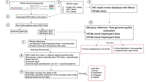
In the Giunta Lab at Sapienza, we typically handle a vast amount of genomic data. Our primary focus is on the de novo assembly of the human diploid genome, a bioinformatics task known for its extensive resource demands in terms of RAM, CPU, and server runtime. The analysis starts with FASTQ files produced from whole-genome sequencing and employs a variety of algorithms to accomplish objectives such as identifying optimal read overlaps, constructing initial graphs, aligning longer reads, generating consensus sequences, final graph creation, and producing FASTA files of the complete genome sequence for each haplotype. The assembled genome's quality is then evaluated using Merqury, a reference-free tool, and Flagger, which flags assembly process inconsistencies for correction, thus enhancing the final assembly's accuracy and completeness. The goal is to complete this resource-intensive process within five days using efficient resource allocation and Slurm, as provided by TeraStat.
Data
Genome assembly relies on whole-genome sequencing data, now greatly improved with third-generation sequencing technologies that provide long reads crucial for spanning potential gaps during overlap. The sequencing data, provided in Fastq format, includes PacBio HiFi reads and ultra-long ONT reads. Phasing of a diploid genome requires a chromatin sequencing method like Hi-C. Quality assessment involves HiFi reads divided into k-mers, evaluated for their frequency and presence in the genome. The assembly outputs include contigs or scaffolds, graphical GFA files, and annotation files detailing genomic features.
Verkko
Input: WGS reads in FASTQ format (.fastq)
Output: Phased assembly in FASTA format (.fasta), assembly graphs in GFA format (.gfa), consensus sequences in FASTA format (.fasta)Meryl and Merqury
Input: HiFi reads in FASTQ format (.fastq)
Output: k-mers HiFi database (.meryl), quality assessment report (.txt or .csv), and visualization files (.png, .pdf, etc.)Flagger
Input: Phased assembly in FASTA format (.fasta), HiFi reads in FASTQ format (.fastq)
Output: k-mers from the genome (.txt), alignment file in BAM format (.bam), alignment index (.bai), and error report in BED format (.bed)Solutions
The TeraStat2 cluster's computational capabilities have significantly reduced the time required to assemble a human diploid genome. By utilizing the pipelines and modules installed on the cluster, we've crafted a streamlined process for de novo genome assembly, integrating wet-lab data directly into the bioinformatics analysis.
Scripts
Here the scripts and server resources used to perform de novo genome assembly and its quality assessment
Download FASTQ raw reads from AWS:
- PacBio CCS: wget 'Download Link 1'
- PacBio CCS: wget 'Download Link 2'
- ONT: wget 'Download Link 3'
- Hi-C: wget 'Download Link 4'
De novo genome assembly tool Verkko:
To run this tool, we need to create a virtual environment with conda:
 module load anaconda/2022.10

			conda create -n verkko

			conda activate verkko

			conda install -c conda-forge -c bioconda -c defaults verkko
Verkko uses a snakemake workflow management allowing a parallelization of each job.Keep the environment activate during Verkko runs:
 Verkko.sh

			#!/bin/sh

			#SBATCH --job-name=verkko #job name

			#SBATCH --output=%x_%j.log #log file name

			#SBATCH --error=%x_%j.err #err file name

			#SBATCH --mem-per-cpu=2G #job memory

			#SBATCH --time=0-100:00:00 #estimated duration

			#SBATCH -n 128 #amount of CPU (s)

			#SBATCH -N 1. #amount of server (s)

			#SBATCH --mail-user=xxx.xxx@uniroma1.it

			#SBATCH --mail-type=ALL
/.conda/envs/lastverkko/bin/verkko -d verkko_phased --slurm \
--hifi *.fastq \
--nano *fastq \
--hic1 *.fastq \
--hic2 *.fastqHere we used command --slurm to ensure that these jobs are scheduled and executed efficiently, maximizing overall throughput, and reducing computation time.
To run:sbatch Verkko.shQuality Evaluation of the De Novo Assembly of Diploid Human Genome
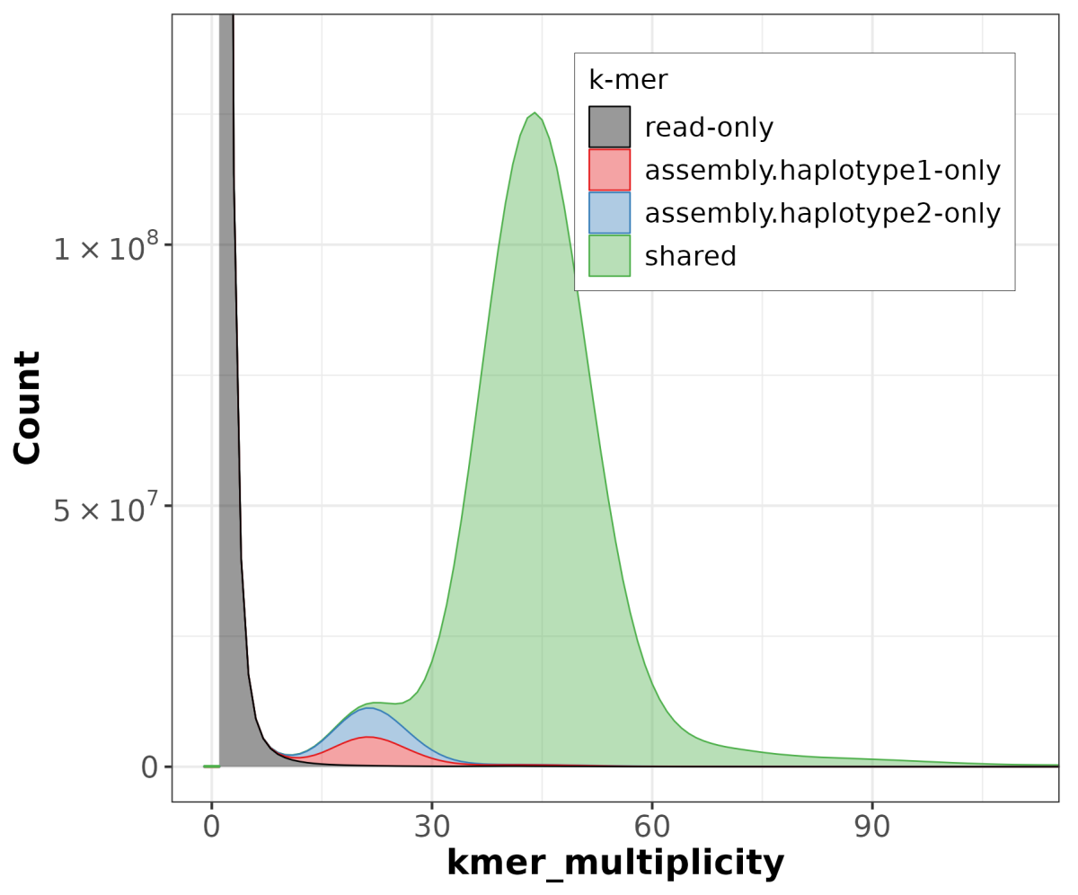
We need to create a set of specific short subsequences from HiFi reads (k-mers) using Meryl. These sets of k-mers will be used to run Merqury, which evaluates genome quality by analyzing the distribution and frequency of k-mers. By comparing the observed k-mer distributions with expected patterns, Merqury provides insights into the accuracy and completeness of the assembly. Higher-quality assemblies typically exhibit consistent and expected k-mer distributions, while lower-quality assemblies may show irregularities. Overall, Merqury helps researchers evaluate the reliability and fidelity of their assembled genomes.
Install Meryl
wget ‘https://github.com/marbl/meryl/releases/tag/v1.4.1’

		tar -xJf meryl-1.4.1.tar.xz

		cd meryl-1.4.1/bin

		export PATH=$PWD:$PATH #Export Meryl path to be available during Merqury run
Install Merqury
wget ‘https://github.com/marbl/merqury/archive/v1.3.tar.gz’

		tar -zxvf v1.3.tar.gz

		cd merqury-1.3

		export MERQURY=$PWD #Set the absolute path of your working directory to use each file or libraries you need to use during Merqury job
These two jobs also require three other tools:
- bedtools
- samtools
- R (to create the final plot)
Reference-free Genome Quality Evaluation Script
To run the Referencefree_genome_quality.sh script, which creates a k-mer database and uses it to estimate the quality of the genome with Merqury, follow these commands:
#!/bin/sh

		#SBATCH --job-name=merqury #job name

		#SBATCH --output=%x_%j.log #log file name

		#SBATCH --error=%x_%j.err #err file name

		#SBATCH --mem-per-cpu=2G #job memory

		#SBATCH -n 128 #amount of CPU (s)

		#SBATCH -N 1 #amount of server (s)

		#SBATCH --time=01:00:00 #estimated duration

		##SBATCH --mail-user=xxx.xxxx@uniroma1.it

		##SBATCH --mail-type=ALL
module load bedtools2/2.30.0_10gcc
module load samtools/1.12_10gcc
module load R/4.2.0_10gcc#Create meryl database with k-mers of specific length, for human k=31
meryl k=31 count output HiFidb.meryl *.fastq.gz# Utilize the k-mers to estimate the quality of the genome
merqury-1.3/merqury.sh /lustre/home/xxx/genome.meryl assembly.hap1.fasta hap1_merqury_graph
assembly.hap2.fasta hap2_merqury_graphTo execute the script:
sbatch Referencefree_genome_quality.shHigh Fidelity Raw Reads Alignment Using Flagger
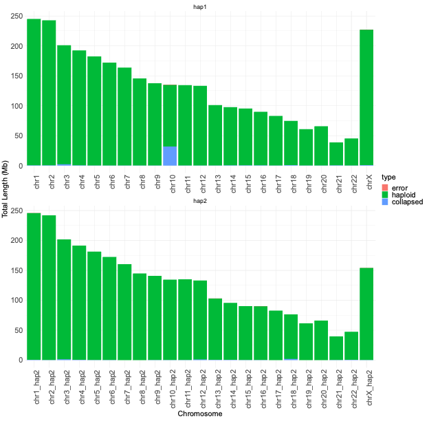
The Flagger tool assesses the quality of each base along the genome by analyzing read alignments. It provides visualizations that indicate error-free regions and identifies potential errors or duplicated sequences.
Install Winnowmap
git clone https://github.com/marbl/Winnowmap.git

		cd Winnowmap

		make -j8
Install Flagger
wget ‘https://github.com/mobinasri/flagger/tree/main/programs/src’

		# from this GitHub page download only the scripts that you need to run
Flagger_genome_evaluation.sh
#!/bin/sh
#SBATCH --job-name=flagger               #job name
#SBATCH --output=%x_%j.log               #log file name
#SBATCH --error=%x_%j.err                #err file name
#SBATCH --mem-per-cpu=2G                 #job memory
#SBATCH --time=0-100:00:00               #amount of CPU (s)
#SBATCH -n 128                           #amount of server (s)
#SBATCH -N 1                             #estimated duration

module load samtools/1.12_10gcc

# K-merize genome
meryl count k=15 output merylDB genome.fasta
meryl print greater-than distinct=0.9998 merylDB > repetitive_k15_genome.txt

# Align HiFi long reads to the genome
winnowmap -W repetitive_k15_genome.txt -ax map-pb -Y -L --eqx --cs -I8g genome.fasta *fastq.gz | \
samtools view -hb | samtools sort -@ 128 > genome.winnowmap.bam
samtools index genome.winnowmap.bam

# Calculate depth of the BAM file
samtools depth -aa -Q 0 genome.winnowmap.bam > genome.depth

# Index the reference
samtools faidx genome.fasta

# Convert the depth file into a coverage file
flagger-0.3.3/programs/src/depth2cov -d genome.depth -f genome.fasta.fai -o genome.cov

# Calculate the frequencies of coverages
cov2counts -i genome.cov -o genome.counts

# Create a table from two-tab delimited .counts output
python fit_gmm.py --counts genome.counts --cov --output genome.table

# Extract blocks (errors, duplicated, collapsed, haploid) from the table
find_blocks_from_table -c genome.cov -t genome.table -p ${OUTPUT_PREFIX
To Run:
sbatch Flagger_genome_evaluation.shConclusions
The computational demands of de novo genome assembly underscore the importance of access to powerful computing resources to facilitate the accurate reconstruction of genomes from sequencing data. We achieved the best performance in terms of job parallelization and run time using Terastat2 resources. The evaluation of genome assembly was done by running Flagger and Merqury, gaining comprehensive insights into the quality and reliability of your genome assembly. The main graphical outputs from these tools provide visual representations of potential errors, accurately assembled regions, and overall assembly quality, enabling you to identify areas for improvement and refine your assembly process.
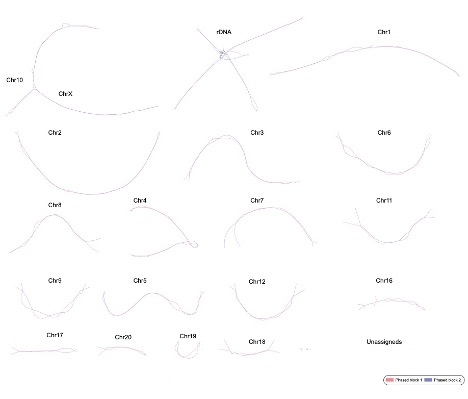
GFA Format Output from Verkko Tool:
- Workshop 2024 Case 4: Consistency of Maximum Likelihood Estimators via EM in relative survival cure models: A large-scale simulation study (Fabrizio Di Mari)
-
Consistency of Maximum Likelihood Estimators via EM in relative survival cure models: A large-scale simulation study
Author
Dott. Fabrizio Di Mari (fabrizio.dimari@uniroma1.it)
Problem Statement
In the frequentist approach, the most commonly used method for estimating a model is to find the Maximum Likelihood estimates of its parameters. However, how can we determine if the output of our implemented precedure is generating the desired estimates? Under mild regularity conditions, among other properties, Maximum Likelihood Estimators are consistent. This means that as the sample size approaches infinity, the estimators tend in probability to the true values of the parameters. Consequently, the Mean Squared Error (MSE) also tends to zero as the sample size increases. Therefore, one method to ensure that we obtain the desired estimates is to conduct a simulation study to verify if the MSE approaches zero as the sample size grows.
Proposed solution
In this case study, we implemented the EM algorithm to obtain the Maximum Likelihood Estimates of a Relative Survival Cure Model. We then assessed whether increasing the sample size also increases the proximity of our estimates to the true values of the model parameters. For each sample size, the algorithm was executed on 250 simulated datasets. Once all 250 estimates were obtained, the mean squared difference across the datasets was computed as an estimate of the MSE. The execution on each separate dataset was parallelized to significantly accelerate the computations. We used to this end the R-package parallel which implements a for loop that distributes iterations among parallel workers.
library(parallel)
# Parameters setting ----
#
tau <- 30*365 # 30 years follow-up
lam0 <- 0.00009 # Scale baseline survival function
beta0 <- 15 # Shape baseline survival function
cp <- 0.08 # censoring proportion
nsim <- 250 # number of simulation
#
# Simulation study ----
source("functions/sim_iter.R")
i <- 1
t0 <- Sys.time()
for (n in c(100, 1000, 10000)){
  if (n == 100){
    cons_check <- as.data.frame(matrix(NA,nrow = 3, ncol = 6))
    row.names(cons_check)<-c("100","1000","10000")
    colnames(cons_check) <- c("bias_cure_probability",
                              "bias_lambda_parameter",
                              "bias_beta_parameter",
                              "MSE_cure_probability",
                              "MSE_lambda_parameter",
                              "MSE_beta_parameter")
  }
  cl <- makeCluster(64, outfile="log/log_workers.txt")
  res <- parLapply(cl,1:nsim,sim_iter,
                   n,tau,cp,lam0,beta0,
                   betad_start=1.5,
                   lamd_start=0.0001,
                   prob0_start=0.4,
                   tol=1e-6)
  stopCluster(cl)
  assign(paste("Res",n,sep = ""),
         matrix(unlist(res), nrow = nsim, ncol = 12,byrow=TRUE),
         env =.GlobalEnv)
  fab <- get(paste("Res",n,sep = ""))
  colnames(fab) <- c("prob0true","prob0","prob0_diff",
                     "lamd_true","lamd","lamd_diff",
                     "betad_true","betad","betad_diff",
                     "diff_last","ll_optim","iter")
  assign(paste("Res",n,sep = ""), fab, env =.GlobalEnv)
  #
  cons_check[i,] <- c(apply(get(paste("Res",n,sep = ""),env=.GlobalEnv),2,mean)[3],# Bias cure probability
                      apply(get(paste("Res",n,sep = ""),env=.GlobalEnv),2,mean)[6],# Bias lambda parameter
                      apply(get(paste("Res",n,sep = ""),env=.GlobalEnv),2,mean)[9],# Bias beta parameter
                      apply(get(paste("Res",n,sep = ""),env=.GlobalEnv)^2,2,mean)[3],# MSE cure probability
                      apply(get(paste("Res",n,sep = ""),env=.GlobalEnv)^2,2,mean)[6],# MSE lambda parameter
                      apply(get(paste("Res",n,sep = ""),env=.GlobalEnv)^2,2,mean)[9])# MSE beta parameter
  i <- i + 1
  cat("End iters for n: ", n,"\n", file="log/log.txt", append = TRUE)
}
#
t1 <- Sys.time() - t0
cat(t1, file="log/log.txt", append = TRUE)
save.image(file="data/res.RData")
#!/bin/sh
#SBATCH --job-name=workshop_sim		    # nome del job nelle code
#SBATCH --output=%x_%j.log          # file di output (stdout)
#SBATCH --error=%x_%j.err           # file di errore (stderr)
#SBATCH --mem-per-cpu=2G            # memoria riservata
#SBATCH --time=0-20:00:00           # riservo per 5 minuti
#SBATCH -n 64                             # amount of cpu(s)
#SBATCH -N 1                                # amount of server(s)
#SBATCH --mail-user=fabrizio.dimari@uniroma1.it
#SBATCH --mail-type=END

module load R

R -f main.R
- Workshop 2024 Case 5: Leverage TeraStat2 to speed up MATLAB Algorithms and Applications (Alessio Conte)
-
Leverage TeraStat2 to speed up MATLAB Algorithms and Applications
Author
Dott. Alessio Conte (aconte@mathworks.com )
Problem
In this talk, an innovative technique will be presented that allows users to leverage MATLAB and the Parallel Computing Toolbox on the multiple cores of TeraStat2 directly from the MATLAB session on the user’s machine, without the need to explicitly log in to TS2 and build scripts with SLURM directives. Nevertheless, it is important to point out that the latter remains always a valid option for using MATLAB on TS2.
After an overview of how this technique works, a case study will be presented. The case study is a readapted version of the example: Analyze Wind Data with Large Compute Cluster in the sense the original dataset has been considerably reduced for demo purposes and made available in the workshop material folder. The dataset is part of the Wind Integration National Dataset Toolkit.
A copy of these instructions is available for download here.
Files and Data
Workshop Material Folder 1 – Scripts and MATLAB-TS2 configuration instructions
Workshop Material Folder 2 – data for wind analysis case study
Folder 1 contains scripts and interactive notebooks used during the workshop. It also contains the instructions for completing the integration of MATLAB with TS2 on the user’s desktop.
Folder 2 contains 3.7 GB of data in case you want to reproduce the wind data analysis case study.
Remote submission to TS2 from MATLAB Desktop
The technique mentioned above leverages a set of publicly available plugin scripts (github.com/mathworks/matlab-parallel-slurm-plugin) that define how your machine communicates with the remote cluster. Participants who want to actively participate and try out the workflows proposed in this workshop should make sure to have completed the MATLAB integration with TS2 prior to the event. Instructions are provided in the workshop material folder.
Below are just a few insights into the workflow; for a more detailed explanation refer to the TS2withMATLAB_1.mlx Live Editor that can be found in the workshop material folder.
function [pi_est, time] = estimatePi(m_points,n_iter)
tic
count = 0;
parfor i = 1:n_iter
    count = count + sum(sum(rand(m_points,2).^ 2,2) < = 1);
end
pi_est = 4/(m_points*n_iter) * count;
time  = toc;
end
The MATLAB code to submit estimatePi to TS2 is:
ts2 = parcluster("TERASTAT2_R2024a"); % create a cluster object
batch(ts2, @estimatePi, 2, {1e6, 1e3}, 'Pool', 16); % submit a batch job
The additional input arguments to the batch function after @estimatePi are, in order, the number of outputs returned by the function (two in this case); a cell array of the inputs; the number of MATLAB workers to run the job on TS2 (actually MATLAB asks 16 + 1 workers, being one the master worker).
To get the results, first get a handle to the job and then fetch the job output:
job = findJob(ts2, 'Name', "estimatePi"); % get a handle to the job
RESULTS = fetchOutputs(job)
Case Study: Analyze Wind Data on TeraStat2
The objective of this case study is to assess the best location for a wind farm starting from the analysis of wind and atmospheric observations for multiple sites. The work presented for this workshop is an adapted version of the example Analyze Wind Data with Large Compute Cluster. Thus, it should be clear that for demo purposes, the original dataset has been considerably reduced, hence results will be different from the original example.
The dataset and code used in this workshop is available in the workshop material folders. The dataset consists of 82 tabular text files each containing atmospheric and wind data measurements for a specific site from 01-January 2007 to 31-December 2013 with a sample interval of 5 minutes (for a total of 736416 observations per file).
Below are just a few insights into the workflow; for a more detailed explanation refer to the wind_data_analysis.mlx Live Editor available in the workshop material folder.
Provided that the "data" folder is available to the user at /lustre/home/username/wind_data_analysis where username is the user account name, the script "batch_process_wind_data" submitted to TS2 is:
windDataStore = fileDatastore("data", 'IncludeSubfolders', true, 'FileExtensions', ".txt", 'ReadFcn', @ReadDs);
pool = gcp;
n_partitions = pool.NumWorkers;
tic
parfor a = 1:n_partitions
ds = partition(windDataStore, n_partitions, a);
store = getCurrentValueStore;
count = 0;
nfilesInPart = length(ds.Files);
while hasdata(ds)
count = count + 1;
t = read(ds);
results = findWindTurbineSite(t);
key = strcat("partition_", num2str(a), " result_", num2str(count));
store(key) = results;
end
end
time = toc;
The key highlight here is the use of datastores to efficient memory management and to partition the dataset for parallel processing across multiple cores. The datastore is partitioned in pool.NumWorkers partitions, corresponding to the number of MATLAB computational engines reserved to this job on TS2 (minus 1 since one is the master worker). Parallel processing of these partitions is instructed with the parallel for loop (parfor). User-defined functions used in this script (ReadDs and findWindTurbineSite) can be found in the workshop material folder. At each iteration, results are stored in a special object known as ValueStore, a versatile mechanism that can be used to pass data between workers and client (in these scenarios, the client is the user's MATLAB desktop).
MATLAB code for submitting the script "batch_process_wind_data" to TS2 on 33 MATLAB workers (one master worker + 32 for the parallel pool):
ts2 = parcluster("TERASTAT2_R2024a");
ts2.AdditionalProperties.WallTime = "00:15:00";
ts2.AdditionalProperties.AdditionalSubmitArgs = "--job-name=wind_data -N 1";
batch(ts2, "batch_process_wind_data", 'Pool', 32, 'CurrentFolder', "/lustre/home/alconte/wind_data_analysis");
After the experiment concludes, results are returned to MATLAB this time using the ValueStore object mentioned earlier. Results, stored on the cluster, can be accessed from the client using a key (similar to dictionaries). For instance, the results of the second file in the third partition processed has the key "partition_3 result_2". Therefore, the code to access this result is:
job_wind_data = findJob(ts2, 'Name', "batch_process_wind_data"); % get job handle
clientStore = job_wind_data.ValueStore; % get the ValueStore object
result = clientStore("partition_3 result_2"); % get specific result for that key
This operation can be performed while the job is running using ValueStore. Once the job is finished all results can be retrieved using the same method, but this time for all keys
clientStore = job_wind_data.ValueStore;
keySet = keys(clientStore);
maxPowerAndKey = cell(1, 2);
for k = 1:length(keySet)
key = keySet{k};
results = clientStore(key);
maxPower = results.powerResults.maxPower;
maxPowerAndKey = compareValue(maxPowerAndKey, {maxPower, key});
end
disp(maxPowerAndKey);
key = maxPowerAndKey{2};
bestSite = clientStore(key);
bestSite = struct with fields:
siteMetadata: [1×1 struct]
checkMissingDate: "No data is missing."
overallData: [1×1 struct]
windDirectionHist: [1×1 struct]
powerResults: [1×1 struct];
- Workshop 2024 Case 6: Containers: an ocean of softwares for NGS data analysis (and everything else) (Giacomo Chiappa)
-
Containers: an ocean of softwares for NGS data analysis (and everything else)
Author
Dott. Giacomo Chiappa (giacomo.chiappa@uniroma1.it)
Problem
From a protein file sequenced from marine gastropods (Source: https://doi.org/10.3390/toxins11110623) we want to filter the input file based on sequence length using the Seqkit package and identify the proteins with a toxin reference database (UniprotKB; https://uniprot.org) using the BLAST package.
All the images .sif files and the experiments .sh scripts are available at the following address.
1. Downloading the images (already available in this folder)
singularity pull docker://pegi3s/seqkit:2.5.1

		singularity pull docker://pegi3s/blast:2.15.0
2. Split long and short peptide sequences
singularity exec seqkit_2.5.1.sif seqkit seq -M 100 Fassioetal2019_peptide.fasta -o Fassioetal2019_short.fasta

		singularity exec seqkit_2.5.1.sif seqkit seq -m 101 Fassioetal2019_peptide.fasta -o Fassioetal2019_long.fasta
Seqkit allows the parsing of genetic sequences files, in our case, we want to filter sequences shorter than 100 amino acids from the others using the seq command. Other information on the usage of this software here: https://bioinf.shenwei.me/seqkit/usage
3. Search for a match in the reference database
singularity exec blast_2.15.0.sif makeblastdb -in uniprotkb_toxin_reference_database.fasta -dbtype prot

		singularity exec blast_2.15.0.sif blastp -query Fassioetal2019_short.fasta -db uniprotkb_toxin_reference_database.fasta -num_threads 32 -max_target_seqs 1 -outfmt 6 -evalue 1e-10 > short_match.list

		singularity exec blast_2.15.0.sif blastp -query Fassioetal2019_long.fasta -db uniprotkb_toxin_reference_database.fasta -num_threads 32 -max_target_seqs 1 -outfmt 6 -evalue 1e-10 > long_match.list
BLAST outputs a table with a line for every match and several pieces of information on the quality of the match in the columns. Other info here: https://angus.readthedocs.io/en/2019/running-command-line-blast.html
The third column gives the percentage identity of the toxin from the Fassio et al. paper with those in the repository. To filter the best results (PID>80) we can use the following command.
awk '$3 > 80 {print $0}' file - Workshop 2024 Case 7: Optimizing Computational Costs in Fluid Dynamics Simulator with Terastat: Scaling Techniques and Applications (Marta Galuppi)
-
Optimizing Computational Costs in Fluid Dynamics Simulator with Terastat: Scaling Techniques and Applications
Author
Dott.ssa Marta Galuppi (marta.galuppi@uniroma1.it)
Problem Statement
The objective of this project is to enhance the computational efficiency of Fire Dynamics Simulator (FDS), a computational fluid dynamics (CFD) model of fire-driven fluid flow, by leveraging TeraStat 2, a High-Performance Computing (HPC) cluster. This improvement will primarily focus on scaling techniques and their practical applications within the FDS framework. FDS is a scientific tool, open source, released by NIST, for simulating fire scenarios in a controlled virtual environment, utilizing a numerical solution of the Navier-Stokes equations suitable for low-speed, thermally driven flow. However, the current computational costs associated with fluid dynamics simulations, particularly concerning large-scale systems or complex fluid behaviours, present significant challenges. By exploiting the capabilities of TS2, an advanced computing platform, the goal is to optimize these costs, facilitating faster and more resource-efficient simulations. This optimization is crucial for enabling detailed analyses of complex fire dynamics, including heat transfer, smoke movement, and structural element interactions, in alignment with observed data from model-scale tests. The iterative process of validating and refining FDS models contributes to the advancement of fire safety research and engineering practices, ultimately promoting the development of more accurate and reliable fire safety strategies. Through this project, we seek to foster safer environments and infrastructure by enhancing the computational efficiency of FDS simulations.
Proposed solution
The commonly used methods rely heavily on domain decomposition techniques, where the computational domain is partitioned into smaller subdomains. These subdomains are then processed independently or semi-independently on various processors of a parallel computer. The coordination among these subdomains is facilitated through synchronized data exchanges. However, it is crucial to ensure that this artificial division does not compromise the inherent global connectivity of the underlying problem. Maintaining the convergence order and approximation quality of the original serial methodology is paramount during the parallelization process. Therefore, meticulous attention must be paid to preserving these characteristics to the highest possible extent.
The following scripts are provided for executing the job related to the previous process statement. To optimize costs, the number of cores for the job must be equal to or greater than the script's mesh requirements. The FDS version used for the job is FDS-6.8.0_SMV-6.8.0.
&HEAD CHID='tunnel', TITLE='Workshop Terastat'  /

//&MISC PARTICLE_CFL=T/

&MESH ID='M_1', IJK=125,25,20, XB=0.0,5.0,0.0,1.0,0.0,0.8/ mesh da 0.04
&MESH ID='M_2', IJK=125,25,20, XB=5.0,10.0,0.0,1.0,0.0,0.8/ mesh da 0.04
&MESH ID='M_3', IJK=125,25,20, XB=10.0,15.0,0.0,1.0,0.0,0.8/ mesh da 0.04
&MESH ID='M_4', IJK=125,25,20, XB=15.0,20.0,0.0,1.0,0.0,0.8/ mesh da 0.04
&MESH ID='M_5', IJK=125,25,20, XB=20.0,25.0,0.0,1.0,0.0,0.8/mesh da 0.04
&MESH ID='M_6', IJK=125,25,20, XB=25.0,30.0,0.0,1.0,0.0,0.8/mesh da 0.04
&MESH ID='M_7', IJK=125,25,20, XB=30.0,35.0,0.0,1.0,0.0,0.8/mesh da 0.04
&MESH ID='M_8', IJK=125,25,20, XB=35.0,40.0,0.0,1.0,0.0,0.8/mesh da 0.04
&MESH ID='M_9', IJK=125,25,20, XB=40.0,45.0,0.0,1.0,0.0,0.8/ mesh da 0.04
&MESH ID='M_10', IJK=125,25,20, XB=45.0,50.0,0.0,1.0,0.0,0.8/ mesh da 0.04
&MESH ID='M_11', IJK=125,25,20, XB=50.0,55.0,0.0,1.0,0.0,0.8/mesh da 0.04
&MESH ID='M_12', IJK=125,25,20, XB=55.0,60.0,0.0,1.0,0.0,0.8/mesh da 0.04

&DUMP DT_RESTART=50./
&MISC RESTART=FALSE./
&COMB EXTINCTION_MODEL='EXTINCTION 2'/

//&PRES VELOCITY_TOLERANCE=1.E-6, MAX_PRESSURE_ITERATIONS=100/

&TIME T_END=570.0 /

&MATL ID='CONCRETE',
      SPECIFIC_HEAT=0.88,
      CONDUCTIVITY=1.37,
      DENSITY=2100.0,
      EMISSIVITY=0.91/
&REAC ID='HEPTANE',
      FUEL='N-HEPTANE',
      CRITICAL_FLAME_TEMPERATURE=1497,
      AUTO_IGNITION_TEMPERATURE=-273.,
      AIT_EXCLUSION_ZONE=0.3,0.6,3.4,3.7,0.8,0.85
      CO_YIELD=0.01,
      SOOT_YIELD=0.037/

&MATL ID='liqHeptane',
      SPECIFIC_HEAT=2.24,
      CONDUCTIVITY=0.125,
      DENSITY=678.0,
      ABSORPTION_COEFFICIENT=301.4,
      HEAT_OF_COMBUSTION=4.809E4,
      HEAT_OF_REACTION=356.0,
      SPEC_ID(1,1)='N-HEPTANE',
      NU_SPEC(1,1)=1.0,
      BOILING_TEMPERATURE=98.38/
&MATL ID='STEEL',
      SPECIFIC_HEAT=0.465,
      CONDUCTIVITY=54.0,
      DENSITY=7833.0,
      EMISSIVITY=0.77/


//&INIT XB=0.0,7.3,3.2,4.0,0.0,8.0, AUTO_IGNITION_TEMPERATURE=-273. /


&DEVC ID='1 NOZ 1.1', XYZ=35.5,0.30,0.45, PROP_ID='Spr1', QUANTITY='CONTROL', CTRL_ID='controller 1', LATCH=.TRUE., ORIENTATION=0,0,-1, /
&DEVC ID='1 NOZ 1.2', XYZ=35.5,0.70,0.45, PROP_ID='Spr1', QUANTITY='CONTROL', CTRL_ID='controller 1', LATCH=.TRUE., ORIENTATION=0,0,-1, /

&DEVC ID='1 NOZ 2.1', XYZ=36.0,0.30,0.45, PROP_ID='Spr1', QUANTITY='CONTROL', CTRL_ID='controller 1', LATCH=.TRUE., ORIENTATION=0,0,-1, /
&DEVC ID='1 NOZ 2.2', XYZ=36.0,0.70,0.45, PROP_ID='Spr1', QUANTITY='CONTROL', CTRL_ID='controller 1', LATCH=.TRUE., ORIENTATION=0,0,-1, /

&DEVC ID='1 NOZ 3.1', XYZ=36.5,0.30,0.45, PROP_ID='Spr1', QUANTITY='CONTROL', CTRL_ID='controller 1', LATCH=.TRUE., ORIENTATION=0,0,-1, /
&DEVC ID='1 NOZ 3.2', XYZ=36.5,0.70,0.45, PROP_ID='Spr1', QUANTITY='CONTROL', CTRL_ID='controller 1', LATCH=.TRUE., ORIENTATION=0,0,-1, /

&DEVC ID='1 NOZ 4.1', XYZ=37.0,0.30,0.45, PROP_ID='Spr1', QUANTITY='CONTROL', CTRL_ID='controller 1', LATCH=.TRUE., ORIENTATION=0,0,-1, /
&DEVC ID='1 NOZ 4.2', XYZ=37.0,0.70,0.45, PROP_ID='Spr1', QUANTITY='CONTROL', CTRL_ID='controller 1', LATCH=.TRUE., ORIENTATION=0,0,-1, /

&DEVC ID='1 NOZ 5.1', XYZ=37.5,0.30,0.45, PROP_ID='Spr1', QUANTITY='CONTROL', CTRL_ID='controller 1', LATCH=.TRUE., ORIENTATION=0,0,-1, /
&DEVC ID='1 NOZ 5.2', XYZ=37.5,0.70,0.45, PROP_ID='Spr1', QUANTITY='CONTROL', CTRL_ID='controller 1', LATCH=.TRUE., ORIENTATION=0,0,-1, /
&DEVC ID='1 NOZ 6.1', XYZ=38.0,0.30,0.45, PROP_ID='Spr1', QUANTITY='CONTROL', CTRL_ID='controller 1', LATCH=.TRUE., ORIENTATION=0,0,-1, /
&DEVC ID='1 NOZ 6.2', XYZ=38.0,0.70,0.45, PROP_ID='Spr1', QUANTITY='CONTROL', CTRL_ID='controller 1', LATCH=.TRUE., ORIENTATION=0,0,-1, /

&DEVC ID='1 NOZ 7.1', XYZ=38.5,0.30,0.45, PROP_ID='Spr1', QUANTITY='CONTROL', CTRL_ID='controller 1', LATCH=.TRUE., ORIENTATION=0,0,-1, /
&DEVC ID='1 NOZ 7.2', XYZ=38.5,0.70,0.45, PROP_ID='Spr1', QUANTITY='CONTROL', CTRL_ID='controller 1', LATCH=.TRUE., ORIENTATION=0,0,-1, /

&DEVC ID='1 NOZ 8.1', XYZ=39.0,0.30,0.45, PROP_ID='Spr1', QUANTITY='CONTROL', CTRL_ID='controller 1', LATCH=.TRUE., ORIENTATION=0,0,-1, /
&DEVC ID='1 NOZ 8.2', XYZ=39.0,0.70,0.45, PROP_ID='Spr1', QUANTITY='CONTROL', CTRL_ID='controller 1', LATCH=.TRUE., ORIENTATION=0,0,-1, /
&DEVC ID='1 NOZ 9.1', XYZ=40.0,0.30,0.45, PROP_ID='Spr1', QUANTITY='CONTROL', CTRL_ID='controller 1', LATCH=.TRUE., ORIENTATION=0,0,-1, /
&DEVC ID='1 NOZ 9.2', XYZ=40.0,0.70,0.45, PROP_ID='Spr1', QUANTITY='CONTROL', CTRL_ID='controller 1', LATCH=.TRUE., ORIENTATION=0,0,-1, /

&DEVC ID='1 NOZ 10.1', XYZ=40.5,0.30,0.45, PROP_ID='Spr1', QUANTITY='CONTROL', CTRL_ID='controller 1', LATCH=.TRUE., ORIENTATION=0,0,-1, /
&DEVC ID='1 NOZ 10.2', XYZ=40.5,0.70,0.45, PROP_ID='Spr1', QUANTITY='CONTROL', CTRL_ID='controller 1', LATCH=.TRUE., ORIENTATION=0,0,-1, /
&DEVC ID='1 NOZ 11.1', XYZ=41.0,0.30,0.45, PROP_ID='Spr1', QUANTITY='CONTROL', CTRL_ID='controller 1', LATCH=.TRUE., ORIENTATION=0,0,-1, /
&DEVC ID='1 NOZ 11.2', XYZ=41.0,0.70,0.45, PROP_ID='Spr1', QUANTITY='CONTROL', CTRL_ID='controller 1', LATCH=.TRUE., ORIENTATION=0,0,-1, /


&DEVC ID='NOZ 1.1', XYZ=41.5,0.30,0.45, PROP_ID='Spr1', QUANTITY='CONTROL', CTRL_ID='controller 1', LATCH=.TRUE., ORIENTATION=0,0,-1, /
&DEVC ID='NOZ 1.2', XYZ=41.5,0.70,0.45, PROP_ID='Spr1', QUANTITY='CONTROL', CTRL_ID='controller 1', LATCH=.TRUE., ORIENTATION=0,0,-1, /

&DEVC ID='NOZ 2.1', XYZ=42.0,0.30,0.45, PROP_ID='Spr1', QUANTITY='CONTROL', CTRL_ID='controller 1', LATCH=.TRUE., ORIENTATION=0,0,-1, /
&DEVC ID='NOZ 2.2', XYZ=42.0,0.70,0.45, PROP_ID='Spr1', QUANTITY='CONTROL', CTRL_ID='controller 1', LATCH=.TRUE., ORIENTATION=0,0,-1, /

&DEVC ID='NOZ 3.1', XYZ=42.5,0.30,0.45, PROP_ID='Spr1', QUANTITY='CONTROL', CTRL_ID='controller 1', LATCH=.TRUE., ORIENTATION=0,0,-1, /
&DEVC ID='NOZ 3.2', XYZ=42.5,0.70,0.45, PROP_ID='Spr1', QUANTITY='CONTROL', CTRL_ID='controller 1', LATCH=.TRUE., ORIENTATION=0,0,-1, /

&DEVC ID='NOZ 4.1', XYZ=43.0,0.30,0.45, PROP_ID='Spr1', QUANTITY='CONTROL', CTRL_ID='controller 1', LATCH=.TRUE., ORIENTATION=0,0,-1, /
&DEVC ID='NOZ 4.2', XYZ=43.0,0.70,0.45, PROP_ID='Spr1', QUANTITY='CONTROL', CTRL_ID='controller 1', LATCH=.TRUE., ORIENTATION=0,0,-1, /

&DEVC ID='NOZ 5.1', XYZ=43.5,0.30,0.45, PROP_ID='Spr1', QUANTITY='CONTROL', CTRL_ID='controller 1', LATCH=.TRUE., ORIENTATION=0,0,-1, /
&DEVC ID='NOZ 5.2', XYZ=43.5,0.70,0.45, PROP_ID='Spr1', QUANTITY='CONTROL', CTRL_ID='controller 1', LATCH=.TRUE., ORIENTATION=0,0,-1, /
&DEVC ID='NOZ 6.1', XYZ=44.0,0.30,0.45, PROP_ID='Spr1', QUANTITY='CONTROL', CTRL_ID='controller 1', LATCH=.TRUE., ORIENTATION=0,0,-1, /
&DEVC ID='NOZ 6.2', XYZ=44.0,0.70,0.45, PROP_ID='Spr1', QUANTITY='CONTROL', CTRL_ID='controller 1', LATCH=.TRUE., ORIENTATION=0,0,-1, /

&DEVC ID='NOZ 7.1', XYZ=44.5,0.30,0.45, PROP_ID='Spr1', QUANTITY='CONTROL', CTRL_ID='controller 1', LATCH=.TRUE., ORIENTATION=0,0,-1, /
&DEVC ID='NOZ 7.2', XYZ=44.5,0.70,0.45, PROP_ID='Spr1', QUANTITY='CONTROL', CTRL_ID='controller 1', LATCH=.TRUE., ORIENTATION=0,0,-1, /

&DEVC ID='NOZ 8.1', XYZ=45.0,0.30,0.45, PROP_ID='Spr1', QUANTITY='CONTROL', CTRL_ID='controller 1', LATCH=.TRUE., ORIENTATION=0,0,-1, /
&DEVC ID='NOZ 8.2', XYZ=45.0,0.70,0.45, PROP_ID='Spr1', QUANTITY='CONTROL', CTRL_ID='controller 1', LATCH=.TRUE., ORIENTATION=0,0,-1, /
&DEVC ID='NOZ 9.1', XYZ=45.5,0.30,0.45, PROP_ID='Spr1', QUANTITY='CONTROL', CTRL_ID='controller 1', LATCH=.TRUE., ORIENTATION=0,0,-1, /
&DEVC ID='NOZ 9.2', XYZ=45.5,0.70,0.45, PROP_ID='Spr1', QUANTITY='CONTROL', CTRL_ID='controller 1', LATCH=.TRUE., ORIENTATION=0,0,-1, /

&DEVC ID='NOZ 10.1', XYZ=46.0,0.30,0.45, PROP_ID='Spr1', QUANTITY='CONTROL', CTRL_ID='controller 1', LATCH=.TRUE., ORIENTATION=0,0,-1, /
&DEVC ID='NOZ 10.2', XYZ=46.0,0.70,0.45, PROP_ID='Spr1', QUANTITY='CONTROL', CTRL_ID='controller 1', LATCH=.TRUE., ORIENTATION=0,0,-1, /
&DEVC ID='NOZ 11.1', XYZ=46.5,0.30,0.45, PROP_ID='Spr1', QUANTITY='CONTROL', CTRL_ID='controller 1', LATCH=.TRUE., ORIENTATION=0,0,-1, /
&DEVC ID='NOZ 11.2', XYZ=46.5,0.70,0.45, PROP_ID='Spr1', QUANTITY='CONTROL', CTRL_ID='controller 1', LATCH=.TRUE., ORIENTATION=0,0,-1, /

&DEVC ID='2 NOZ 1.1', XYZ=47.0,0.30,0.45, PROP_ID='Spr1', QUANTITY='CONTROL', CTRL_ID='controller 1', LATCH=.TRUE., ORIENTATION=0,0,-1, /
&DEVC ID='2 NOZ 1.2', XYZ=47.0,0.70,0.45, PROP_ID='Spr1', QUANTITY='CONTROL', CTRL_ID='controller 1', LATCH=.TRUE., ORIENTATION=0,0,-1, /

&DEVC ID='2 NOZ 2.1', XYZ=47.5,0.30,0.45, PROP_ID='Spr1', QUANTITY='CONTROL', CTRL_ID='controller 1', LATCH=.TRUE., ORIENTATION=0,0,-1, /
&DEVC ID='2 NOZ 2.2', XYZ=47.5,0.70,0.45, PROP_ID='Spr1', QUANTITY='CONTROL', CTRL_ID='controller 1', LATCH=.TRUE., ORIENTATION=0,0,-1, /

&DEVC ID='2 NOZ 3.1', XYZ=48.0,0.30,0.45, PROP_ID='Spr1', QUANTITY='CONTROL', CTRL_ID='controller 1', LATCH=.TRUE., ORIENTATION=0,0,-1, /
&DEVC ID='2 NOZ 3.2', XYZ=48.0,0.70,0.45, PROP_ID='Spr1', QUANTITY='CONTROL', CTRL_ID='controller 1', LATCH=.TRUE., ORIENTATION=0,0,-1, /

&DEVC ID='2 NOZ 4.1', XYZ=48.5,0.30,0.45, PROP_ID='Spr1', QUANTITY='CONTROL', CTRL_ID='controller 1', LATCH=.TRUE., ORIENTATION=0,0,-1, /
&DEVC ID='2 NOZ 4.2', XYZ=48.5,0.70,0.45, PROP_ID='Spr1', QUANTITY='CONTROL', CTRL_ID='controller 1', LATCH=.TRUE., ORIENTATION=0,0,-1, /

&DEVC ID='2 NOZ 5.1', XYZ=49.0,0.30,0.45, PROP_ID='Spr1', QUANTITY='CONTROL', CTRL_ID='controller 1', LATCH=.TRUE., ORIENTATION=0,0,-1, /
&DEVC ID='2 NOZ 5.2', XYZ=49.0,0.70,0.45, PROP_ID='Spr1', QUANTITY='CONTROL', CTRL_ID='controller 1', LATCH=.TRUE., ORIENTATION=0,0,-1, /
&DEVC ID='2 NOZ 6.1', XYZ=49.5,0.30,0.45, PROP_ID='Spr1', QUANTITY='CONTROL', CTRL_ID='controller 1', LATCH=.TRUE., ORIENTATION=0,0,-1, /
&DEVC ID='2 NOZ 6.2', XYZ=49.5,0.70,0.45, PROP_ID='Spr1', QUANTITY='CONTROL', CTRL_ID='controller 1', LATCH=.TRUE., ORIENTATION=0,0,-1, /

&DEVC ID='2 NOZ 7.1', XYZ=50.0,0.30,0.45, PROP_ID='Spr1', QUANTITY='CONTROL', CTRL_ID='controller 1', LATCH=.TRUE., ORIENTATION=0,0,-1, /
&DEVC ID='2 NOZ 7.2', XYZ=50.0,0.70,0.45, PROP_ID='Spr1', QUANTITY='CONTROL', CTRL_ID='controller 1', LATCH=.TRUE., ORIENTATION=0,0,-1, /

&DEVC ID='2 NOZ 8.1', XYZ=50.5,0.30,0.45, PROP_ID='Spr1', QUANTITY='CONTROL', CTRL_ID='controller 1', LATCH=.TRUE., ORIENTATION=0,0,-1, /
&DEVC ID='2 NOZ 8.2', XYZ=50.5,0.70,0.45, PROP_ID='Spr1', QUANTITY='CONTROL', CTRL_ID='controller 1', LATCH=.TRUE., ORIENTATION=0,0,-1, /
&DEVC ID='2 NOZ 9.1', XYZ=51.0,0.30,0.45, PROP_ID='Spr1', QUANTITY='CONTROL', CTRL_ID='controller 1', LATCH=.TRUE., ORIENTATION=0,0,-1, /
&DEVC ID='2 NOZ 9.2', XYZ=51.0,0.70,0.45, PROP_ID='Spr1', QUANTITY='CONTROL', CTRL_ID='controller 1', LATCH=.TRUE., ORIENTATION=0,0,-1, /

&DEVC ID='2 NOZ 10.1', XYZ=51.5,0.30,0.45, PROP_ID='Spr1', QUANTITY='CONTROL', CTRL_ID='controller 1', LATCH=.TRUE., ORIENTATION=0,0,-1, /
&DEVC ID='2 NOZ 10.2', XYZ=51.5,0.70,0.45, PROP_ID='Spr1', QUANTITY='CONTROL', CTRL_ID='controller 1', LATCH=.TRUE., ORIENTATION=0,0,-1, /
&DEVC ID='2 NOZ 11.1', XYZ=52.0,0.30,0.45, PROP_ID='Spr1', QUANTITY='CONTROL', CTRL_ID='controller 1', LATCH=.TRUE., ORIENTATION=0,0,-1, /
&DEVC ID='2 NOZ 11.2', XYZ=52.0,0.70,0.45, PROP_ID='Spr1', QUANTITY='CONTROL', CTRL_ID='controller 1', LATCH=.TRUE., ORIENTATION=0,0,-1, /

&SPEC ID='WATER VAPOR SPK', SPEC_ID='WATER VAPOR'/
&SPEC ID='WATER VAPOR'/

&PROP ID='Spr1', QUANTITY='SPRINKLER LINK TEMPERATURE', FLOW_RATE=0.016, PART_ID='water_drops', K_FACTOR=0.0063, SPRAY_PATTERN_TABLE='TABLE1', PARTICLES_PER_SECOND=1000. /
&PART ID='water_drops', SPEC_ID='WATER VAPOR', SAMPLING_FACTOR=10, QUANTITIES='PARTICLE DIAMETER', DIAMETER= 19./

&TABL ID='TABLE1', TABLE_DATA=12.5,92.5,0.0,65.0,15.79,0.2/
&TABL ID='TABLE1', TABLE_DATA=12.5,92.5,72.0,137.0,15.79,0.2/
&TABL ID='TABLE1', TABLE_DATA=12.5,92.5,144.0,209.0,15.79,0.2/
&TABL ID='TABLE1', TABLE_DATA=12.5,92.5,216.0,281.0,15.79,0.2/
&TABL ID='TABLE1', TABLE_DATA=12.5,92.5,288.0,353.0,15.79,0.2/

&SLCF QUANTITY='VOLUME FRACTION', SPEC_ID='WATER VAPOR', PBY=3.4/
&SLCF QUANTITY='VOLUME FRACTION', SPEC_ID='WATER VAPOR SPK', PBY=3.4/
&SLCF PBY=3.4, QUANTITY='oxygen' /

&DEVC XYZ=0.1,0.1,0.1, ID='clock 1', QUANTITY='TIME'/

&CTRL ID='controller 1', FUNCTION_TYPE='CUSTOM', INPUT_ID='clock 1', RAMP_ID='ramp 1', LATCH=.FALSE. /

&RAMP ID='ramp 1', T= 0.00, F=-1. /
&RAMP ID='ramp 1', T= 23.00, F=-1. /
&RAMP ID='ramp 1', T= 24.00, F=1. / da verificare se usare questo o la stringa successiva
==&CTRL ID='controller 1', FUNCTION_TYPE='DEADBAND', SETPOINT=23.0,84.0, ON_BOUND='UPPER', LATCH=.FALSE., INPUT_ID='temp37'/


&SURF ID='BURNER', HRRPUA=387.0, TAU_Q=-60.0, COLOR='RED', E_COEFFICIENT=1 /

&SURF ID='CAR',
      COLOR='WHITE',
      BACKING='VOID',
      MATL_ID(1,1)='STEEL',
      MATL_MASS_FRACTION(1,1)=1.0,
      THICKNESS(1)=0.05/


&SURF ID='CLS PARETI',
      COLOR='GRAY 80',
      BACKING='VOID',
      MATL_ID(1,1)='CONCRETE',
      MATL_MASS_FRACTION(1,1)=1.0,
      THICKNESS(1)=0.15,
      ROUGHNESS=0.01/

&OBST ID='Obstruction #1', XB=0.0,60.0,0.0,0.1,0.0,0.8, SURF_ID='CLS PARETI'/
&OBST ID='Obstruction #2', XB=0.0,60.0,0.9,1.0,0.0,0.8, SURF_ID='CLS PARETI'/
&OBST ID='Obstruction #3', XB=0.0,60.0,0.8,0.9,0.4,0.8, SURF_ID='CLS PARETI'/
&OBST ID='Obstruction #4', XB=0.0,60.0,0.1,0.2,0.4,0.8, SURF_ID='CLS PARETI'/
&OBST ID='Obstruction #5', XB=0.0,60.0,0.2,0.3,0.5,0.8, SURF_ID='CLS PARETI'/
&OBST ID='Obstruction #6', XB=0.0,60.0,0.7,0.8,0.5,0.8, SURF_ID='CLS PARETI'/
&OBST ID='Obstruction #7', XB=0.0,60.0,0.3,0.4,0.6,0.8, SURF_ID='CLS PARETI'/
&OBST ID='Obstruction #8', XB=0.0,60.0,0.6,0.7,0.6,0.8, SURF_ID='CLS PARETI'/
&OBST ID='Obstruction #9', XB=0.0,60.0,0.4,0.6,0.7,0.8, SURF_ID='CLS PARETI'/
&OBST ID='Obstruction #9', XB=0.0,60.0,0.0,1.0,0.0,0.1, SURF_ID='CLS PARETI'/


&OBST ID='car1', XB=39.0,40.0,0.1,0.4,0.1,0.2, SURF_ID='CAR'/
&VENT ID='burner', SURF_ID='BURNER', XB=39.5,40.0,0.1,0.26,0.2,0.2/
&VENT ID='burner', SURF_ID='OPEN', XB=30.0,40.0,0.8,0.9,0.0,0.0/

&VENT ID='XMIN', SURF_ID='OPEN', XB=0.0,0.0,0.0,1.0,0.0,0.8/
&VENT ID='XMAX', SURF_ID='OPEN', XB=60.0,60.0,0.0,1.0,0.0,0.8/


&BNDF QUANTITY='GAUGE HEAT FLUX' /
&BNDF QUANTITY='NET HEAT FLUX'/
&BNDF QUANTITY='WALL TEMPERATURE'/
&SLCF PBY=0.5, QUANTITY='TEMPERATURE' /


&DUMP DT_DEVC=10.0/
&DEVC ID='temp01', QUANTITY='TEMPERATURE', XYZ=10.0,0.5,0.2/
&DEVC ID='temp02', QUANTITY='TEMPERATURE', XYZ=20.0,0.5,0.2/
&DEVC ID='temp03', QUANTITY='TEMPERATURE', XYZ=30.0,0.5,0.2/
&DEVC ID='temp04', QUANTITY='TEMPERATURE', XYZ=40.0,0.5,0.2/
&DEVC ID='temp05', QUANTITY='TEMPERATURE', XYZ=50.0,0.5,0.2/
&DEVC ID='temp06', QUANTITY='TEMPERATURE', XYZ=60.0,0.5,0.2/


&DEVC ID='vis01', QUANTITY='VISIBILITY', XYZ=10.0,0.5,0.2/
&DEVC ID='vis02', QUANTITY='VISIBILITY', XYZ=20.0,0.5,0.2/
&DEVC ID='vis03', QUANTITY='VISIBILITY', XYZ=30.0,0.5,0.2/
&DEVC ID='vis04', QUANTITY='VISIBILITY', XYZ=40.0,0.5,0.2/
&DEVC ID='vis05', QUANTITY='VISIBILITY', XYZ=50.0,0.5,0.2/
&DEVC ID='vis06', QUANTITY='VISIBILITY', XYZ=60.0,0.5,0.2/


&DEVC ID='CO01', QUANTITY='VOLUME FRACTION', SPEC_ID='CARBON MONOXIDE', XYZ=10.0,0.5,0.2/
&DEVC ID='CO02', QUANTITY='VOLUME FRACTION', SPEC_ID='CARBON MONOXIDE', XYZ=20.0,0.5,0.2/
&DEVC ID='CO03', QUANTITY='VOLUME FRACTION', SPEC_ID='CARBON MONOXIDE', XYZ=30.0,0.5,0.2/
&DEVC ID='CO04', QUANTITY='VOLUME FRACTION', SPEC_ID='CARBON MONOXIDE', XYZ=40.0,0.5,0.2/
&DEVC ID='CO05', QUANTITY='VOLUME FRACTION', SPEC_ID='CARBON MONOXIDE', XYZ=50.0,0.5,0.2/
&DEVC ID='CO06', QUANTITY='VOLUME FRACTION', SPEC_ID='CARBON MONOXIDE', XYZ=60.0,0.5,0.2/


&DEVC ID='COdue01', QUANTITY='VOLUME FRACTION', SPEC_ID='CARBON DIOXIDE', XYZ=10.0,0.5,0.2/
&DEVC ID='COdue02', QUANTITY='VOLUME FRACTION', SPEC_ID='CARBON DIOXIDE', XYZ=20.0,0.5,0.2/
&DEVC ID='COdue03', QUANTITY='VOLUME FRACTION', SPEC_ID='CARBON DIOXIDE', XYZ=30.0,0.5,0.2/
&DEVC ID='COdue04', QUANTITY='VOLUME FRACTION', SPEC_ID='CARBON DIOXIDE', XYZ=40.0,0.5,0.2/
&DEVC ID='COdue05', QUANTITY='VOLUME FRACTION', SPEC_ID='CARBON DIOXIDE', XYZ=50.0,0.5,0.2/
&DEVC ID='COdue06', QUANTITY='VOLUME FRACTION', SPEC_ID='CARBON DIOXIDE', XYZ=60.0,0.5,0.2/


&DEVC ID='IRR01', QUANTITY='INTEGRATED INTENSITY', XYZ=10.0,0.5,0.2/
&DEVC ID='IRR02', QUANTITY='INTEGRATED INTENSITY', XYZ=20.0,0.5,0.2/
&DEVC ID='IRR03', QUANTITY='INTEGRATED INTENSITY', XYZ=30.0,0.5,0.2/
&DEVC ID='IRR04', QUANTITY='INTEGRATED INTENSITY', XYZ=40.0,0.5,0.2/
&DEVC ID='IRR05', QUANTITY='INTEGRATED INTENSITY', XYZ=50.0,0.5,0.2/
&DEVC ID='IRR06', QUANTITY='INTEGRATED INTENSITY', XYZ=60.0,0.5,0.2/


&DEVC ID='t01', QUANTITY='TEMPERATURE', XYZ=10.0,0.5,0.6/
&DEVC ID='t02', QUANTITY='TEMPERATURE', XYZ=20.0,0.5,0.6/
&DEVC ID='t03', QUANTITY='TEMPERATURE', XYZ=30.0,0.5,0.6/
&DEVC ID='t04', QUANTITY='TEMPERATURE', XYZ=40.0,0.5,0.6/
&DEVC ID='t05', QUANTITY='TEMPERATURE', XYZ=50.0,0.5,0.6/
&DEVC ID='t06', QUANTITY='TEMPERATURE', XYZ=60.0,0.5,0.6/


&SLCF PBY=0.5, QUANTITY='VELOCITY', VECTOR=T, CELL_CENTERED=T /

&TAIL /
(click here to download the source code)
Scripts
#!/bin/sh
#SBATCH --job-name=tunnel10wm.fds             # work_name
#SBATCH --mem-per-cpu=2G                # memoria riservata
#SBATCH --time=0-100:00:00                 #riservo per 100 ore
#SBATCH -n 16                                # numero di core
#SBATCH -N 2                                # numero di nodes
#SBATCH --mail-user=marta.galuppi@uniroma1.it
#SBATCH --mail-type=ALL
export OMP_NUM_THREADS=12

module load FDS6
fds tunnel10wm.fds
- Workshop 2024 Case 8: Study of the Protein Structural Dynamics in Solution (Alessandro Nardi, Giuseppe Chen)
-
Containers: an ocean of softwares for NGS data analysis (and everything else)
Author
Dott. Alessandro Nardi, Dott. Giuseppe Chen (alessandro.nardi@uniroma1.it)
Problem
Classical molecular dynamics (MD) simulations are nowadays among the most commonly used computational techniques to obtain information about the structural dynamics of condensed phase systems. The Gromacs software package is an efficient and versatile program that allows performing classical MD simulations of proteins and nucleic acids in solution. Gromacs offers the possibility of extensive (CPU and GPU) parallelization that speeds up bottleneck calculations. In this demonstration, we will exploit the CPU parallelization offered by Gromacs on TeraStat2. The performance of TS2 will be tested for the dynamics of a small-sized protein in aqueous solution, as a case study. Additionally, the typical analyses performed on an MD trajectory will be shown.
Solution
A copy of the materials used for this case study is available for download here
- Workshop 2024 Case 9: Benchmarking computational topology tools using interactive jobs (Riccardo Ceccaroni)
-
Benchmarking computational topology tools using interactive jobs
Author
Dott. Riccardo Ceccaroni (fabrizio.dimari@uniroma1.it)
Problem Statement
Frequently, we encounter multiple software implementations for tackling the same problem, prompting the need to identify the most efficient option. This scenario is evident in the computation of persistent homology, a method for computing topological features of a space at different spatial resolutions. Numerous software solutions have emerged for this purpose. This study focuses on software designed to extract topological features from images, with a specific interest in zero-dimensional persistent homology achieved through simplicial complex filtering. Two options for this task are Ripser, renowned for its stability and versatility, and the newly developed PixHomology.
Solutions
To determine the most efficient solution in terms of execution time and memory usage, we propose a benchmarking approach on Terastat2 utilizing interactive jobs (TS2) for real-time results. The script used is
test.pywhich calculates the memory and execution time of the software on the dataset specified at startup. Below is the step-by-step guide to create the environment on TS2 and run the script.0. Connect to TS2
Accessing TS2 involves establishing a connection to the login node through the ssh text terminal. The command from the terminal is:
bash ssh -l user_name -p 2020 ts2.uniroma1.itwhereuser_nameis the personal username assigned to you after the access request. For more details see https://dss.uniroma1.it/it/HPCTeraStat2/Collegarsi.1. Workspace Setup:
In this section, our objective is to establish a directory on the Terastat platform encompassing all essential files indispensable for comprehensively engaging with the tutorial.
1.1 Clone the GitHub repository
To clone the GitHub repository means to create a local copy of a repository hosted on GitHub on your machine. This allows you to access the files, commit changes, and collaborate with others. The necessary command to accomplish this is typically
git clone <repository_URL>. The repository URL for this tutorial is https://github.com/example/repository.git, the command would be:git clone https://github.com/riccardoc95/TS2BenchmarkThis command will download all the files from the specified repository into a directory named after the repository on your local machine.
1.2 Change the working directory
Navigate to the working directory refers to changing the current directory in the command line interface to the directory where you want to perform actions or execute commands. This can be achieved using the
cdcommand followed by the directory path. The working directory is named TS2Benchmark, the command is:bash cd TS2BenchmarkThis command would switch the current directory to TS2Benchmark within the home directory, allowing you to carry out tasks within that specific directory.2. Setup Conda Environment
TS2 provides a set of products and software libraries of general interest. Among these, we find the conda package manager. To activate the module just execute the command:
bash module load anacondaWhen executed, this command loads the Anaconda module, which is a distribution of the Python (and/or R) programming language along with additional packages and tools commonly used in scientific computing, data science, and machine learning. Loading the Anaconda module ensures that the Anaconda distribution and its associated tools are available for use within the current environment (including the conda command), enabling users to easily access Python and its associated libraries for their computational tasks.After loading the form you will need to restart your session. You can terminate and rerun the
sshsession or executebash source ~/.bashrc2.1 Create a new Python environment:
Since the packages already present in the Conda distribution are not sufficient and we need to install others and since modifying the base environment is restricted in Conda/Anaconda, we opt to create a fresh environment. This can be achieved using the following command:
bash conda create -n ts2b python=3.11This creates a new Conda environment named ts2b with Python version 3.11.To use the new environment we must activate it with:
bash conda activate ts2bWhen activated, this environment becomes the primary environment for executing commands and running Python scripts within the current terminal session.3 Python packages
Now we can proceed with installing the packages. There are several methods to install Python packages, each with its own advantages and use cases. Here are the most common methods:
3.1 Using pip (Python Package Installer):
pip is the default package manager for Python. To install a package using pip, you can use
pip install package_name. For example, we need to install the Ripser package. The command is:bash pip install ripserFor installing multiple packages at once we can use a requirements file. Therequirements.txtfile typically contains a list of package names. To install using pip, you can use:bash pip install -r requirements.txtATTENTION: Also Conda is a package manager for Python. It is particularly useful for managing Python environments and installing packages with dependencies. To install a package using Conda, you can use the following command
conda install package_name. However, not all Python packages are managed by conda.3.2 From Source
Sometimes, you may want to install a package directly from its source code. This happens when a package is not present on pip or you need a different version than the one managed by pip. This involves downloading the source code from the package's repository and running the setup script to install it. For example, PixHomology package is not yet on pip. We can download its source code with:
bash git clone https://github.com/riccardoc95/PixHomology cd PixHomologyAs compiling the source code requires specific development tools, we rely on TS2 to provide these tools. However, to access them, we must load the necessary modules. Specifically, we require a C compiler and the CMake utility. This can be accomplished using the following commands:bash module load gcc module load cmakeThe commands to install from source may vary depending on the package, but typically involve running:bash pip install .After install, we return to our working directory with:
bash cd ..4. Download of datasets
To download datasets refers to acquiring data files from a remote location, typically over the internet, for use in analysis, research, or other purposes. This process involves retrieving the data files from a source and saving them to a local storage location. Depending on the source and the data format, various methods can be employed for downloading datasets.
-
Download manually:
bash
bashcd datawget -c "https://www.dropbox.com/scl/fi/ol2v2u36zoqdm2j4xsyvu/MNIST.zip?rlkey=ea0ckamg4fbiff60njughkf69&dl=0" -O MNIST.zipwget -c "https://www.dropbox.com/scl/fi/059zdeiisypqek314rdvk/CIFAR10.zip?rlkey=tjrgvejepx6i8ajjhqxghr8k2&dl=0" -O CIFAR10.zipunzip MNIST.zipunzip CIFAR10.ziprm MNIST.ziprm CIFAR10.zipcd ..-
With python script:
bash python dataset.py
5. Executing the job within an interactive shell
Executing a task within an interactive shell is accomplished using the
sruncommand, which is typically employed in high-performance computing environments for job submission and management. Below is an example of how to run a job interactively usingsrun:srun -N 1 -n 1 -p dss -t 00:30:00 --pty /bin/bashwhere: -
srun: Initiates the submission of a job to the scheduler. --N 1: Specifies that the job should be allocated resources on 1 compute node. --n 1: Requests 1 CPU cores for the job. --p dss: Assigns the job to the dss partition in the cluster, which typically schedules jobs that can fit into gaps in the regular scheduling queue. --t 00:30:00: Sets a time limit of 30 minutes for the job to execute. ---pty: Requests a pseudo-terminal for the job, enabling interactive access. -/bin/bash: Specifies the shell (in this case, Bash) to be used for the interactive session once the job starts running.ATTENTION: it is possible that the environment will disappear when you switch to the terminal of the new machine. To reset it:
bash conda activate ts2bUpon running this command, users gain access to an interactive shell session where they can execute commands, run programs, and perform other tasks within the allocated computing environment. This interactive session persists until the user exits the shell or the allocated resources reach their specified limits.
We run
benchmark.shwith:chmod +x benchmark.sh ./benchmark.sh -
Download manually:
- Esempio parallelizzazione in R
-
Esempio parallelizzazione in R
Riportiamo qui un esempio di utilizzo della libreria doParallel di R per prarallelizzare parte di un algoritmo di stima del valore del pi greco.
Per questa stima viene utilizzato il metodo Monte Carlo. Si considera un quadrato di lato 1 con un cerchio inscritto. Il rapporto delle aree del quadrato e del cerchio è proporzionale a Pi. Si distribuisono poi casualmente sul quadrato dei punti. Il rapporto tra il numero di punti distributi sul quadrato e quello dei punti che finiscono all'interno del cerchio inscritto sarà proporzionale, per grandi numeri di tentativi, al rapporto tra le aree e, quindi, a pi greco.
Una implementazione sequenziale di questo algoritmo è:
library(ggplot2)

			library(scales)
nCicli <- 6
nStime <- 64
nPunti <- 1df <- data.frame( NumPunti=integer(), stima=double(), std=double(), time=double() )
for ( ciclo in 1:nCicli ){
start_time <- Sys.time()
nPunti <- nPunti * 10stime <- vector()
for ( stima in 1:nStime ){
nIn=0for ( step in 1:nPunti ) {
x=runif(1,0,1)
y=runif(1,0,1)
if( x*x+y*y <= 1 ){
nIn=nIn+1
}
}stime <- c( stime, 4*nIn/nPunti)
}
end_time <- Sys.time()
df <- rbind( df, data.frame( NumPunti=nPunti, stima=mean(stime), std=sd(stime),
time=end_time-start_time ) ) }
print(df)
p <- ggplot(df,aes(x = NumPunti, y= stima)) +
geom_point() +
geom_pointrange( aes( ymin=stima-std, ymax=stima+std))
p + scale_x_log10()ggsave("PiPlot_seq.pdf")In questa implementazione, attraverso dei cicli, lo script ripete la stima numerose volte e con differenti numeri di punti casuali (da 1 a 1 milione); nello specifico vengono effettuate 64 stime per ognuno di 6 valori differenti del numero di punti.
Premesso che questo algoritmo è particolarmente adatto alla parallelizzazione in quanto le varie stime sono indipendenti l'una dall'altra, bisogna comunque individuare delle sottoprocedure che siano anche abbastanza corpose da giustificare l'inevitabile sovraccarico del controllo della parallelizzazione.
Per effettuare la parallelizzazione la libreria che andremo ad utilizzare (doParallel) permette di definire un pool di processi worker a cui verrà affidata l'esecuzione delle sottoprocedure e, attraverso delle speciali direttive nei cicli di R permette di indicare quali parti del programma devono essere delegate e parallelizzate. Ad esempio se si dispone di 10 worker e il ciclo prevede 100 passi la libreria farà si che i primi 10 passi vengano affidati ai processi worker e mano a mano che un worker termina il proprio lavoro, comunica il risultato al processo padre che gli affida il passo successivo fino al completamento del ciclo.
La prima cosa da fare è quindi modificare lo script di schedulazione assicurandosi di avere risorse a sufficienza per eseguire i processi worker:
#!/bin/sh#SBATCH --job-name=stima_Pi_par # nome del job
#SBATCH --output=%x_32_%j.log # nome del file di output
#SBATCH --error=%x_32_%j.err # nome del file di errore
#SBATCH --mem-per-cpu=1G # memoria richiesta
#SBATCH --time=0-00:40:00 # tempo esecuzione richiesto (giorni-ore:minuti:secondi)
#SBATCH -n 32 # numero di processori da utilizzare
#SBATCH -N 1 # numero di server da utilizzare
#SBATCH --mail-user=utente@esempio.es # proprio indirizzo email
#SBATCH --mail-type=ENDmodule load R
R --slave -f stimaPi_par.Rdove si vede che con la direttiva -n 32 vengono richiesti 32 core.
La versione parallelizzata della procedura diventa:
library(doParallel)

			library(ggplot2)

			library(scales)
num_cores <- as.numeric(Sys.getenv("SLURM_CPUS_ON_NODE"))
registerDoParallel(cores = num_cores)nCicli <- 6
nStime <- 64
nPunti <- 1df <- data.frame( NumPunti=integer(), stima=double(), std=double(), time=double() )
for ( ciclo in 1:nCicli ){
start_time <- Sys.time()
nPunti <- nPunti * 10stime = foreach ( stima=1:nStime, .combine='c' ) %dopar% {
nIn <- 0
for( step in 1:nPunti) {
x=runif(1,0,1)
y=runif(1,0,1)
if( x*x+y*y <= 1 ){
nIn = nIn+1
}
}
4*nIn/nPunti
}
end_time <- Sys.time()
df <- rbind( df, data.frame( NumPunti=nPunti, stima=mean(stime), std=sd(stime),
time=as.numeric(end_time-start_time,units="secs") ) )
}print(df)
p <- ggplot(df,aes(x = NumPunti, y= stima)) +
geom_point() +
geom_pointrange( aes( ymin=stima-std, ymax=stima+std))
p + scale_x_log10()ggsave(paste("PiPlot_",num_cores,".pdf", sep=""))Oltre all'inclusione della libreria scelta per la parallelizzazione si può vedere che viene indicato alla libreria doParallel il numero di core disponibili; infatti le due righe
 num_cores <- as.numeric(Sys.getenv("SLURM_CPUS_ON_NODE"))

registerDoParallel(cores = num_cores)leggono dall'ambiente di esecuzione il numero di core riservati sul nodo e utilizzano questa informazione per inizializzare il pool di worker.
Il ciclo foreach, il cui blocco calcolo la singola stima di ogni ciclo, tramite la direttiva %dopar% indica alla libreria che il blocco di codice deve essere esguito da uno dei woker.
- Workshop 2022 Case 2: Efficient multiple input handling using R (Marco Mingione)
-
Efficient multiple input handling using R
Author
Dott. Marco Mingione (marco.mingione@uniroma1.it)
Problem Statement
In many real-world data applications, there is a need to process and analyze input data that is originally distributed across multiple (possibly huge) files.
The natural solution would be to read these files sequentially and merge them in a single data object for later analysis. However, such an approach is unefficient as it requires an execution time that is linear in the size of the input.
Solutions
We exploit the distributed nature of TeraStat2 by developing a procedure in R for reading in parallel the content of several data files by using multiple processors. We use to this end several parallelization packages available with R and pre-installed on TeraStat 2 like: foreach, doParallel, multicore.
We consider, as case-study a dataset reporting hourly data about waves height and direction in the South Mediterranean from January to October 2022.
Parallel solution
 1
 2
 3
 4
 5
 6
 7
 8
 9
10
11
12
13
14
15
16
17
18
19
20
21
22
23
24
25
26
27
28
29
30
31
32
33
34
35
36
37
38
39
40
#!/usr/bin/env Rscript
args = commandArgs(trailingOnly=TRUE)

# Load packages
packs <- c("tidyverse", "magrittr", "lubridate", "doParallel", "foreach")
suppressMessages(suppressWarnings(sapply(packs, require, character.only = T)))

# Data
rdata_files <- list.files("data/", full.names = T, pattern = ".RData")
n_files <- as.numeric(args[1])
#n_files <- 10
Ntimes <- 24 # hourly data

# get number of cores
n_cores <- detectCores()
cl <- makeCluster(n_cores-2) # create cluster and is good practice to leave some threads free
t0 <- Sys.time() # save initial time
final_dat <- foreach(fl = 1:length(rdata_files[1:n_files]), .combine = bind_rows, .inorder = T, .packages = "tidyverse") %dopar% {
  # Load the ith RData file
  load(rdata_files[fl])
  # Create part of the output
  coords_hour <- expand_grid(lat = data$lat, lon = data$lon, date_time = data$time) %>% arrange(date_time, lat, lon)
  hm0 <- lapply(1:Ntimes, function(i) as.vector(data$hm0[,,i])) %>% reduce(c)
  mdr <- lapply(1:Ntimes, function(i) as.vector(data$mdr[,,i])) %>% reduce(c)
  oo <- coords_hour %>% mutate(hm0 = hm0, mdr = mdr)
  return(oo)
  rm(coords_hour, hm0, mdr)
}
print("Final computation time is: ")
(t1 <- Sys.time() - t0) # save final time
stopCluster(cl) # stop cluster

print("Final object size is: ")
print(object.size(final_dat), units = "Mb")

# final_dat %>% filter(date_time == min(date_time)) %>% ggplot(aes(x = lon, y = lat, color = hm0)) + geom_point()
#
# final_dat %>% drop_na %>% filter(lon == lon[1], lat == lat[1]) %>% ggplot(aes(x = date_time, y = hm0)) + geom_line()
# final_dat %>% drop_na %>% filter(lon %in% lon[1:100], lat %in% lat[1:100]) %>%
#   ggplot(aes(x = date_time, y = hm0, group = interaction(lon,lat))) + geom_line()
(click here to download the source code)
We provide as well the code required to implement a traditional approach to this problem, by reading the different files sequentially.
Sequential solution
 1
 2
 3
 4
 5
 6
 7
 8
 9
10
11
12
13
14
15
16
17
18
19
20
21
22
23
24
25
26
27
28
29
30
31
32
33
34
35
36
37
#!/usr/bin/env Rscript
args = commandArgs(trailingOnly=TRUE)

# Load packages
packs <- c("tidyverse", "magrittr", "lubridate")
suppressMessages(suppressWarnings(sapply(packs, require, character.only = T)))

# Dati
rdata_files <- list.files("data/", full.names = T, pattern = ".RData")
n_files <- as.numeric(args[1])
#n_files <- 10
Ntimes <- 24

final_dat <- list() # output list
t0 <- Sys.time() # save initial time
for(fl in rdata_files[1:n_files]){
  # Load the ith RData file
  load(fl)
  # Create part of the output
  coords_hour <- expand_grid(lat = data$lat, lon = data$lon, date_time = data$time) %>% arrange(date_time, lat, lon)
  hm0 <- lapply(1:Ntimes, function(i) as.vector(data$hm0[,,i])) %>% reduce(c)
  mdr <- lapply(1:Ntimes, function(i) as.vector(data$mdr[,,i])) %>% reduce(c)
  final_dat[[fl]] <- coords_hour %>% mutate(hm0 = hm0, mdr = mdr)
  rm(coords_hour, hm0, mdr)
}
final_dat %<>% reduce(bind_rows)
print("Final computation time is: ")
(t1 <- Sys.time() - t0) # save final time

print("Final object size is: ")
print(object.size(final_dat), units = "Mb")

# final_dat %>% filter(date_time == min(date_time)) %>% ggplot(aes(x = lon, y = lat, color = hm0)) + geom_point()
#
# final_dat %>% drop_na %>% filter(lon == lon[1], lat == lat[1]) %>% ggplot(aes(x = date_time, y = hm0)) + geom_line()
# final_dat %>% drop_na %>% filter(lon %in% lon[1:100], lat %in% lat[1:100]) %>%
#   ggplot(aes(x = date_time, y = hm0, group = interaction(lon,lat))) + geom_line()
(click here to download the source code)
Data
Hourly data for waves height and direction in the South Mediterranean from January 1st to January 31th. One file for each day, for a total of 31 files.
Each file contains an R object called data and including:
- 2 arrays, one for wave height and one for wave direction, each of dimension 361 × 192 × 24 (lon × lat × hour)
- a vector of length 361 with the distinct longitudes
- a vector of length 192 with the distinct latitudes
- a vector of length 24 with the distinct hours
Click here to download the whole dataset (one single ZIP file of approx. 400MB)
Scripts
In the following we report some examples of script files useful for executing either the parallel or the sequential version of the code we proposed on the previously mentioned data. In both cases, we first load the TeraStat 2 module needed for using version 4.0.5 of R and, then, launch our experiment by specifying the R file to be executed together with its parameters
Note: all the SBATCH directives (line 2-10) should be changed at your convenience.
Script for executing the parallel version
 1
 2
 3
 4
 5
 6
 7
 8
 9
10
11
12
13
#!/bin/sh
#SBATCH --job-name="parallel_30"              # jobname
#SBATCH --output=%x_%j.log            # output file
#SBATCH --error=%x_%j.err                # error file
#SBATCH --time=0-01:00:00                 # estimated duration
#SBATCH --mem-per-cpu=2GB               # amount of memory per cpu
#SBATCH -n 30                             # amount of cpu(s)
#SBATCH -N 1                                # amount of server(s)
#SBATCH --mail-user=john.doe@uniroma1.it
#SBATCH --mail-type=ALL

module load R/4.0.5_10gcc
Rscript --vanilla parallel.R 30
(click here to download the source code)
 1
 2
 3
 4
 5
 6
 7
 8
 9
10
11
12
13
#!/bin/sh
#SBATCH --job-name="sequential"              # jobname
#SBATCH --output=%x_%j.log            # output file
#SBATCH --error=%x_%j.err                # error file
#SBATCH --time=0-01:00:00                 # estimated duration
#SBATCH --mem-per-cpu=2GB               # amount of memory per cpu
#SBATCH -n 1                             # amount of cpu(s)
#SBATCH -N 1                                # amount of server(s)
#SBATCH --mail-user=john.doe@uniroma1.it
#SBATCH --mail-type=ALL

module load R/4.0.5_10gcc
Rscript --vanilla sequential.R 30
- Workshop 2022 Case 4: Simulation and analysis of protein dynamics in unconventional solvents (Leonardo Guidoni)
-
Simulation and analysis of protein dynamics in unconventional solvents
Author
prof. Leonardo Guidoni
Problem Statement
Gromacs is one among the most efficient and versatile program to simulate molecular dynamics of liquids, proteins and nucleic acids. In this short demonstration we see how to start and analyze a molecular dynamic simulation of a small protein embedded in an unconventional chemical solvent: a mixture of water and Deep Eutectic Solvent (DES).
Solution
A molecular dynamic simulation needs 3 main file categories:
- A file (or more files) containing the topology and the force-field. For the protein we used standard amber force-field. For the DES molecules we used an adapted version of the gaff force-field. Gromacs tools used: pdb2gmx.
- A file containing the starting coordinates. The starting coordinates of the simulation box has been obtained by solvating a lysozyme protein with a pre- equilibrated mixture of water and DES. Gromacs tool used: grompp, mdrun.
- Input file for energy minimization and molecular dynamics. Two files are used. The first (run0.mdp) for initial optimization, the second (run1.mdp).
Data
Input files
- Topology and related files (*.top, *.itp)
- Starting coordinate file (*.gro)
- Input files (*.mdp)
- Index file for data analysis (*.ndx)
Scripts
Script for execution of the parallel version:
 1
 2
 3
 4
 5
 6
 7
 8
 9
10
11
12
13
14
15
#!/bin/sh
#SBATCH --job-name=test_gromacs # nome del job nelle code
#SBATCH --output=%x_%j.log # file di output
#SBATCH --error=%x_%j.err # file di errore
#SBATCH --mem-per-cpu=1024M # memoria riservata
#SBATCH --time=1-00:0:00 # riservo per 1 minuto
#SBATCH -n 32 # numero di core
#SBATCH -N 1 # numero di nodes
#SBATCH --mail-user=
#SBATCH --mail-type=ALL

module load gromacs/2021.3_10gcc

gmx_mpi grompp -f run0.mdp -c starting_coordinates.gro -p topol.top -o run0.tpr
gmx_mpi mdrun -s run0.tpr -deffnm test_gromacs -maxh 24.0
- Workshop 2022 Case 5: Parallel Human Genome Data Analysis (Luca Corda)
-
Parallel Human Genome Data Analysis
Authors:
- Luca Corda: luca.corda@uniroma1.it
- Simona Giunta: simona.giunta@uniroma1.it
- Lab Email: GiuntaLab@gmail.com
Problem Statement
Biological samples are often acquired in batch, generating big data that need to be processed and analyzed simultaneously. To study multiple data by processing them for multi-parameters acquisition, the most time-efficient and reproducible way is to run the same script on each file in parallel. In the Giunta Lab at Sapienza, we routinely generate large amount of genomic data through sequencing experiments that require computation post-processing of samples through custom-made pipelines, as shown in the example below.
Solutions
The architecture of TeraStat2 cluster allows us to perform our analysis in very few steps directly using the modules already installed in the cluster. By developing a procedure in bash and using specific tools, it is possible to analyze genomic data in parallel using our custom pipelines. Here, I am presenting as proof-of-principle, a basic pipeline to evaluate CENP-A enriched regions of the human genome starting from publicly available ChIP-Seq data and the latest human reference genome assembly:

Data
A common type of sequencing-derived genomic data are fastq files. These are text files containing all the DNA sequence information. When these raw files are mapped to a reference sequence, which can be an en-tire genome or portions of it, they become BAM files. Here, we use sequencing data derived from a chromatin immuno-precipitation experiment (ChIP-seq) to investigate the binding of a protein to DNA and its enrichment on specific regions of the genome. We illustrate in this example the spread of Centromeric Protein A (CENP-A) on specific regions of the genome, and test whether our pipeline shows enriched peaks of this protein where we would expect, namely at human centromere.
INPUT: multiple human ChIP sequencing fastq files and a reference fasta file.OUTPUT: for each input file, a binary alignment map (.bam) file, an index file (.bai) and a coverage track file (.bigwig) will be generated.
Scripts
This section reports some examples of script files written in bash useful to perform the ChIP-seq analysis in parallel.
Warning: Standard TeraStat 2 accounts come with a 100GB disk space availability. In order to perform the following experiments, you will have to ask the system administrator for an upgrade of your disk capacity otherwise the experiments will fail for lack of disk space.
Download data from NCBI (sra toolkit):
This step allows to obtain public data of ChIP-seq experiments that we will use as input for the analysis. It takes advantage of the download.sh script shown below to download a collection of paired-end reads starting from their id.
1
2
3
4
5
#!/bin/sh

module load sratoolkit/3.0.1 #load SRA Toolkit module

fastq-dump --split-files $1  #download paired-end reads given by the SRA id in list.txt
(click here to download the script)
We used this script to download the paired-end fastq files for each of the 4 experiments:
- Input 1 of CHM13hTERT (36GB) <- https://www.ncbi.nlm.nih.gov/sra/SRX9708460 [accn]
- Input 2 of CHM13hTERT (38GB) <- https://www.ncbi.nlm.nih.gov/sra/SRX9708461 [accn]
- CENP-A 1 ChIP-Seq of CHM13hTERT (42GB) <- https://www.ncbi.nlm.nih.gov/sra/SRX9708458 [accn]
- CENP-A 2 ChIP-Seq of CHM13hTERT (48GB) <- https://www.ncbi.nlm.nih.gov/sra/SRX9708459 [accn]
Thus, we first created a text file called list.txt containing the id of all paired-end reads collections to download
1
2
3
4
SRR13278681
SRR13278682
SRR13278683
SRR13278684
(click here to download the file)
Then, we executed the following command from the command-line to download all collections described in list.txt
1
for i in `cat list.txt`; do bash download.sh $i; done
Note: when run on TeraStat 2, this script requires about 10 hours to download all the input files.
Quality check (fastqc)
Data quality check is one of the most important steps in human genomic data analysis. Here, I describe the way we use FastQC, the software that provides the quality report on our starting raw data and allow us to move on to the next step in the shortest possible time, because of the parallel running of these jobs. The output of the FastQC tool is an html report with various information about the reads, such as base sequence quality, sequence duplication levels, adapter content and others. In our case, we take advantage of the many cores available with TeraStat 2 by running FastQC with the help of the fastqc.sh script shown below:
 1
 2
 3
 4
 5
 6
 7
 8
 9
10
11
12
13
14
#!/bin/sh
#SBATCH --job-name=fastqc                                   #job name
#SBATCH --output=%x_%j.log                                  #log file name
#SBATCH --error=%x_%j.err                                   #err file name
#SBATCH --mem-per-cpu=2G                                    #job memory
#SBATCH -n 128                                              #amount of CPU (s)
#SBATCH -N 1                                                #amount of server (s)
#SBATCH --time=02:00:00                                     #estimated duration
#SBATCH --mail-user=john.doe@uniroma1.it
#SBATCH --mail-type=ALL

module load fastqc/0.11.9  #load FastQC module

fastqc --threads 128 $1    #parallel quality control analysis
(click here to download the script)
The fastqc.sh script is executed, turnwise, on all fastq files downloaded before using the following command line:
1
for i in *fastq; do sbatch fastqc.sh $i; done
Note: when run on TeraStat 2, this step requires about 10 minutes to analyze all the input files.
Genome index (bwa index)
The human reference genome we consider in these experiments, t2t-chm13-v2.0.fa.gz, can be retrieved from the following address:
http://t2t.gi.ucsc.edu/chm13/hub/t2t-chm13-v2.0/genome/?C=M;O=DIt can be downloaded in one shot by executing the following command:
1
wget http://t2t.gi.ucsc.edu/chm13/hub/t2t-chm13-v2.0/genome/t2t-chm13-v2.0.fa.gz
The downloaded genome is indexed using the bwa_index.sh script described below:
 1
 2
 3
 4
 5
 6
 7
 8
 9
10
11
12
13
14
15
#!/bin/sh
#SBATCH --job-name=index                     #job name
#SBATCH --output=%x_%j.log                   #log file name
#SBATCH --error=%x_%j.err                    #err file name
#SBATCH --mem-per-cpu=2G                     #job memory
#SBATCH -n 128                               #amount of CPU (s)
#SBATCH -N 1                                 #amount of server (s)
#SBATCH --time=02:00:00                      #estimated duration
#SBATCH --mail-user=john.doe@uniroma1.it
#SBATCH --mail-type=ALL

module load python/3.9.2_10gcc #load the python module
module load bwa/0.7.17         #load the BWA module

bwa index -a bwtsw -p chm13.v2.0 t2t-chm13-v2.0.fa.gz #index reference genome
(click here to download the script)
Note: when run on TeraStat 2, this step requires about 1 hour to analyze the input file.
Alignment (bwa mem and samtools)
Burrows-Wheeler Aligner (bwa) is a software package that performs mapping sequences against a large reference, such as the human genome. With this script it is possible to map all our fastq files in parallel against the large sequence of our choice. In this case we will map to the T2T human reference genome and this step will take between 0.5h and 2h of time to complete. Once completed, we will have our raw Binary Alignment Map (BAM) file.
 1
 2
 3
 4
 5
 6
 7
 8
 9
10
11
12
13
14
15
16
#!/bin/sh
#SBATCH --job-name=alignment                                #job name
#SBATCH --output=%x_%j.log                                  #log file name
#SBATCH --error=%x_%j.err                                   #err file name
#SBATCH --mem-per-cpu=2G                                    #job memory
#SBATCH -n 128                                              #amount of CPU (s)
#SBATCH -N 1                                                #amount of server (s)
#SBATCH --time=90:00:00                                     #estimated duration
#SBATCH --mail-user=john.doe@uniroma1.it
#SBATCH --mail-type=ALL

module load python/3.9.2_10gcc  #load the python module
module load bwa/0.7.17          #load the BWA module
module load samtools/1.12_10gcc #load the Samtools module

bwa mem chm13.v2.0 $1\_1.fastq $1\_2.fastq -t 128 | samtools view -bSh - > $1\.bam #alignment and SAM > BAM conversion
(click here to download the script)
Alignment is performed according to all collections of paired-end reads reported in list.txt, by executing the following command:
1
for i in `cat list.txt`; do sbatch alignment.sh $i; done
Note: when run on TeraStat 2, this step requires about 2 hours to analyze all the input files.
Processing (samtools)
The processing of the BAM files is useful to obtain a more reliable data. It is possible to filter the mapped reads in different ways, in the following script, named filter.sort.sh, we remove the unmapped reads, the secondary alignments and the supplementary alignments. Additionally, we can also sort the BAM files to order them and also reduce them to a smaller size.
 1
 2
 3
 4
 5
 6
 7
 8
 9
10
11
12
13
14
15
#!/bin/sh
#SBATCH --job-name=filter                                      #job name
#SBATCH --output=%x_%j.log                                     #log file name
#SBATCH --error=%x_%j.err                                      #err file name
#SBATCH --mem-per-cpu=2G                                       #job memory
#SBATCH -n 128                                                 #amount of CPU (s)
#SBATCH -N 1                                                   #amount of server (s)
#SBATCH --time=90:00:00                                        #estimated duration
#SBATCH --mail-user=john.doe@uniroma1.it
#SBATCH --mail-type=ALL

module load samtools/1.12_10gcc #load samtools module

samtools view -h -F 0x904 $1 | samtools sort -@ 128 - -O BAM -o $1\.filter.sort.bam      #sort by chromosome
samtools index $1\.filter.sort.bam                                                       #index bam file
(click here to download the script)
The filter.sort.sh script is run on all bam files using the following command line:
1
for i in *bam; do sbatch filter.sort.sh $i; done
Note: when run on TeraStat 2, this step requires about 10 minutes to analyze all the input files.
Coverage track (deeptools)
This tool takes an alignment of reads or fragments as input (BAM file) and generates a coverage track (bigWig or bedGraph) as output.
The coverage is calculated as the number of reads per bin, where bins are short consecutive counting windows of a defined size.1 2 3 4 5 6 7 8 9 10 11 12 13 14 15
#!/bin/sh #SBATCH --job-name=coverage #job name #SBATCH --output=%x_%j.log #log file name #SBATCH --error=%x_%j.err #err file name #SBATCH --mem-per-cpu=2G #job memory #SBATCH -n 128 #amount of CPU (s) #SBATCH -N 1 #amount of server (s) #SBATCH --time=05:00:00 #estimated duration #SBATCH --mail-user=john.doe@uniroma1.it #SBATCH --mail-type=ALL module load python/3.9.2_10gcc #load the python module module load deeptools/ #load the deepTools module bamCoverage -b $1 -o $1\.bw --binSize 10 --normalizeUsing RPGC --effectiveGenomeSize 3000000000 #create track coverage files
(click here to download the script)
Type this command to run the script:
1
for i in *filter.sort.bam; do sbatch coverage.sh $i; done
Note: when run on TeraStat 2, this step requires about 40 minutes to analyze all the input files.
Conclusion
After the ChIP-seq data analysis, we can obtain a graphical visualization of the peak files which show the coverage of mapped reads along the reference genome using the Integrative Genome Viewer (IGV) tool. After the alignment of raw reads to the genome and data filtering, it is now possible to identify enriched signal regions (peak calling) of our protein of interest. We can choose to visualize the spread of our protein along the entire chromosome or narrow down with a zoom in into our regions of interest. Figure below shows an example of the entire chromosome 5:
- Workshop 2022 Case 6: Parallel Monte Carlo Markov Chain with JAGS and R (Gianmarco Caruso)
-
Parallel Monte Carlo Markov Chain with JAGS and R
Authors
Dott. Gianmarco Caruso (gianmarco.caruso@uniroma1.it)
Problem Statement
We consider a simple context in which we want to estimate the parameters (intercept, slope, and variance of errors) of a simple linear regression model. The parameters are estimated in a Bayesian framework exploiting Monte Carlo Marko Chains (MCMCs) via the well-known Bayesian program JAGS (which can be used in R). To evaluate the ability of the method to recover the true value of the model parameter, we consider a simulation study where K datasets are simulated using the same model specification and the true model is fitted to each of the K replicas.
Solutions
We show how parallelization, while fitting the K-replicas, provides a significant efficiency gain over the classical sequential solution. Moreover, parallelization is also possible within each single model fitting, e.g., by running parallel chains. Finally, we provide some summaries to evaluate the performance of the model.We work with simulated data. Details on the simulation setup can be found in the following simSetting.R script.Parallel solution
fitParallel.R
1 2 3 4 5 6 7 8 9 10 11 12 13 14 15 16 17 18 19 20 21 22 23 24 25 26 27 28 29 30 31 32
source("simSetting.R") #run the script with the simulation setting require(R2jags) require(doParallel) # FIT A SIMPLE LINEAR MODEL ON EACH REPLICAS (PARALLEL SOLUTION) ncores = detectCores() # get number of cores available on the machine cl = makeCluster(ncores-2) # create cluster doParallel::registerDoParallel(cl) start.time = Sys.time() # save initial time fit_parallel = foreach(k = 1:K, .inorder = T, .packages = "R2jags") %dopar% { #jags.parallel parallelises over the number of chains jags.parallel(data = list("x"=sim_data[[k]]$x, "y"=sim_data[[k]]$y), inits = start.values, parameters.to.save = c("beta0","beta1","sigma"), model.file = "simplereg.txt", n.chains = nc, n.iter = niter, n.burnin = nburnin, n.thin = thin) } print("Final computation time is: ") (parallel_time = Sys.time() - start.time) stopCluster(cl) # stop cluster
(click here to download the source code)
We provide as well the code required to implement a traditional approach to this problem.
Sequential solution
fitSequential.R
1 2 3 4 5 6 7 8 9 10 11 12 13 14 15 16 17 18 19 20 21 22 23 24 25 26 27 28 29 30
source("simSetting.R") #run the script with the simulation setting require(R2jags) # FIT A SIMPLE LINEAR MODEL ON EACH REPLICAS (SEQUENTIAL SOLUTION) start.time = Sys.time() # save initial time fit_sequential = vector("list",K) for(k in 1:K){ #jags.parallel parallelises over the number of chains fit_sequential[[k]] = jags.parallel(data = list("x"=sim_data[[k]]$x, "y"=sim_data[[k]]$y), inits = start.values, parameters.to.save = c("beta0","beta1","sigma"), model.file = "simplereg.txt", n.chains = nc, n.iter = niter, n.burnin = nburnin, n.thin = thin, export_obj_names = c("nc","niter","nburnin","thin")) } print("Final computation time is: ") (parallel_time = Sys.time() - start.time)
(click here to download the source code)
The Bayesian model
simplereg.txt
1 2 3 4 5 6 7 8 9 10 11 12 13 14 15 16 17 18 19 20 21
model{ #Priors beta0 ~ dnorm(0,0.001) #intercept beta1 ~ dnorm(0,0.001) #slope sigma ~ dunif(0,100) #standard deviation tau = 1/sigma^2 #precision #Likelihood for( i in 1:length(y)){ y[i] ~ dnorm(beta0 + beta1*x[i], tau) #NB argument of dnorm() are the mean and the precision (i.e. precision=1/variance) } }(click here to download the source code)
Data
We use for this experiment simulated data, as returned by the simSetting.R code shown above.
1 2 3 4 5 6 7 8 9 10 11 12 13 14 15 16 17 18 19 20 21 22 23 24 25 26 27 28 29 30 31 32 33 34 35 36 37 38 39 40 41 42 43 44 45 46
#We consider a simple linear regression model: #y = beta0 + beta1*x + epsilon, where epsilon ~ Normal(0, sigma). #Given n observations (x_i, y_i), we want to obtain a Bayesian estimation (via MCMC implemented in JAGS) of the model's parameters: beta0, beta1 and sigma. # WRITE THE FUNCTION TO SIMULATES VALUES FOR INDEPENDENT AND DEPENDENT VARIABLES ---- sim.slreg = function(n, beta0, beta1, sigma){ x = rnorm(n, 175, 7) y = beta0 + beta1*x + rnorm(n,0,sigma) return(as.data.frame(cbind(x=x, y=y))) } # DETAILS OF THE EXPERIMENT ---- n = 100 #number of units in each dataset beta0 = -50 #intercept beta1 = 0.7 #slope sigma = 3 #standard deviation of the error # SIMULATING REPLICAS ---- K = 100 #number of replicated datasets set.seed(123) #setting a seed for sim_data = replicate(K, simplify = FALSE, sim.slreg(n, beta0, beta1, sigma)) # BUILD A FUNCTION WHICH SIMULATES A LIST OF STARTING VALUES FOR EACH CHAIN ---- start.values = function(){ beta0 = runif(1,-200,200) beta1 = runif(1,-50,50) sigma = runif(1,0,10) list(beta0=beta0, beta1=beta1, sigma=sigma) } # DETAILS OF THE MCMC RUN ---- nc = 2 #number of chains niter = 1e5 #total number of iterations for each chain nburnin = niter/2 #the first half of the iterations is discarded thin = 1 #no thinning
Scripts
In the following we report some examples of script files useful for executing either the parallel or the sequential version of the code we proposed on the previously mentioned data. In both cases, we first load the TeraStat 2 module needed for using version 4.0.5 of R and, then, launch our experiment by specifying the R file to be executed together with its parameters
Note: all the SBATCH directives (line 2-8) should be changed at your convenience.
Script for executing the parallel version
1 2 3 4 5 6 7 8 9 10 11 12
#!/bin/sh #SBATCH --job-name="parallel" # jobname #SBATCH --output=%x_%j.log # output file #SBATCH --error=%x_%j.err # error file #SBATCH --time=0-01:00:00 # estimated duration #SBATCH --mem-per-cpu=2GB # amount of memory per cpu #SBATCH -n 30 # amount of cpu(s) #SBATCH -N 1 # amount of server(s) module load jags module load R Rscript --vanilla fitParallel.R
(click here to download the script)
Script for executing the sequential version
1 2 3 4 5 6 7 8 9 10 11 12
#!/bin/sh #SBATCH --job-name="sequential" # jobname #SBATCH --output=%x_%j.log # output file #SBATCH --error=%x_%j.err # error file #SBATCH --time=0-01:00:00 # estimated duration #SBATCH --mem-per-cpu=2GB # amount of memory per cpu #SBATCH -n 1 # amount of cpu(s) #SBATCH -N 1 # amount of server(s) module load jags module load R Rscript --vanilla fitSequential.R
(click here to download the script)
Output
Once the experiment will be finished, it will be possible to evaluate the performance of the model using the following code.
1 2 3 4 5 6 7 8 9 10 11 12 13 14 15 16 17 18 19 20 21 22 23 24 25 26 27 28 29 30 31 32 33 34 35 36 37 38 39 40 41 42 43 44 45 46 47 48 49 50 51 52 53 54 55 56 57 58 59 60 61 62 63 64 65 66 67 68 69
load("outParallel.RData")
#load("outSequential.RData") #same content as outParallel.RData

require(HDInterval) #we load a package useful for computing HPD credible interval

# ANALYSING THE CONTENT OF THE FIRST REPLICA ----

fit_parallel[[1]]$BUGSoutput #posterior summaries for the first replica

beta0_d1 = fit_parallel[[1]]$BUGSoutput$sims.matrix[,"beta0"]
beta1_d1 = fit_parallel[[1]]$BUGSoutput$sims.matrix[,"beta1"]
sigma_d1 = fit_parallel[[1]]$BUGSoutput$sims.matrix[,"sigma"]

hdi(beta0_d1, credMass = 0.95)
hdi(beta1_d1, credMass = 0.95)
hdi(sigma_d1, credMass = 0.95)

par(mfrow=c(2,3))
#estimated posterior densities
hist(beta0_d1); abline(v=beta0, col=2)
hist(beta1_d1); abline(v=beta1, col=2)
hist(sigma_d1); abline(v=sigma, col=2)
#traceplots
plot(beta0_d1,type="l"); abline(h=beta0, col=2)
plot(beta1_d1,type="l"); abline(h=beta1, col=2)
plot(sigma_d1,type="l"); abline(h=sigma, col=2)

summary(lm(y~x, data = sim_data[[1]])) #comparing with the solution obtained in the frequentist framework

# BRIEF ANALYSIS OF THE PERFORMANCE OVER THE K REPLICAS ----

## Posterior estimates

#NB. We excluded the third column which refers to the chain of the 'deviance'

post_means = sapply(fit_parallel,
                    function(x) colMeans(x$BUGSoutput$sims.matrix[,-3]))

par(mfrow=c(1,3))
boxplot(post_means["beta0",], main=expression(hat(beta)[0])); abline(h=beta0, col=2)
boxplot(post_means["beta1",], main=expression(hat(beta)[1])); abline(h=beta1, col=2)
boxplot(post_means["sigma",], main=expression(hat(sigma))); abline(h=sigma, col=2)

## Credible intervals and coverage

CI95_beta0 = sapply(fit_parallel,
                    function(x) hdi(x$BUGSoutput$sims.matrix[,"beta0"], credMass = 0.95))
CI95_beta1 = sapply(fit_parallel,
                    function(x) hdi(x$BUGSoutput$sims.matrix[,"beta1"], credMass = 0.95))
CI95_sigma = sapply(fit_parallel,
                    function(x) hdi(x$BUGSoutput$sims.matrix[,"sigma"], credMass = 0.95))

covCI95_beta0 = mean(apply(CI95_beta0, 2, function(x) beta0>x[1] & beta0<x[2]))
covCI95_beta1 = mean(apply(CI95_beta1, 2, function(x) beta1>x[1] & beta1<x[2]))
covCI95_sigma = mean(apply(CI95_sigma, 2, function(x) sigma>x[1] & sigma<x[2]))

par(mfrow=c(1,3))

plot(0,0, xlim=c(min(CI95_beta0), max(CI95_beta0)), ylim=c(0,K), xlab=expression(beta[0]), ylab="replica", main=paste("coverage=",covCI95_beta0))
for(i in 1:K) segments(CI95_beta0[1,i],i,CI95_beta0[2,i],i, col=3)
abline(v=beta0, col=2)

plot(0,0, xlim=c(min(CI95_beta1), max(CI95_beta1)), ylim=c(0,K), xlab=expression(beta[1]), ylab="replica", main=paste("coverage=",covCI95_beta1))
for(i in 1:K) segments(CI95_beta1[1,i],i,CI95_beta1[2,i],i, col=4)
abline(v=beta1, col=2)

plot(0,0, xlim=c(min(CI95_sigma), max(CI95_sigma)), ylim=c(0,K), xlab=expression(sigma), ylab="replica", main=paste("coverage=",covCI95_sigma))
for(i in 1:K) segments(CI95_sigma[1,i],i,CI95_sigma[2,i],i, col=6)
abline(v=sigma, col=2)
- Workshop 2022 Case 7: Scaling Intensive Calculations in Matlab: Applications (Mathworks)
-
Scaling Intensive Calculations in MATLAB: Applications
Requirements
Before trying to run these experiments, follow the directions provided in https://www.dss.uniroma1.it/it/HPCTeraStat2/IntegrazioneMatlab about configuring a Matlab installation to work with TeraStat 2.
Problem Statement
This workshop will explore the solutions of three problems using parallel computing: Monte Carlo simulation to solve the birthday paradox, Solutions of the Van Der Pol Oscillator and Training a Classification Model for X-Ray Chest Images.
Solution
Download the workshop_parallelcomputing. file, extract its content with MATLAB and follow the instructions inside the workshop_script.mlx file.
Data
NIH Chest X-ray Dataset, which can be found here:
https://www.kaggle.com/
datasets/nih-chest-xrays/data Scripts
No scripts are needed for these experiments as their execution on TeraStat 2 is automatically instrumented by Matlab, provided that the initial configuration has been completed.